steven_yang thesis

NAVAL

POSTGRADUATE SCHOOL

MONTEREY, CALIFORNIA

THESIS

Further dissemination only as directed by President, Code 261 (September 2012) Naval Postgraduate School, Monterey,

CA 93943–5000, or DoD authority.

EXPERIMENTAL VERIFICATION OF THE ACOUSTIC RADIATION FORCE

by

Steve Yang

September 2012

Thesis Advisor: B. Denardo Second Reader: G. Karunasiri

THIS PAGE INTENTIONALLY LEFT BLANK

i

REPORT DOCUMENTATION PAGE Form Approved OMB No. 0704–0188 Public reporting burden for this collection of information is estimated to average 1 hour per response, including the time for reviewing instruction, searching existing data sources, gathering and maintaining the data needed, and completing and reviewing the collection of information. Send comments regarding this burden estimate or any other aspect of this collection of information, including suggestions for reducing this burden, to Washington headquarters Services, Directorate for Information Operations and Reports, 1215 Jefferson Davis Highway, Suite 1204, Arlington, VA 22202–4302, and to the Office of Management and Budget, Paperwork Reduction Project (0704–0188) Washington DC 20503. 1. AGENCY USE ONLY (Leave blank)

2. REPORT DATE September 2012

3. REPORT TYPE AND DATES COVERED Master’s Thesis

4. TITLE AND SUBTITLE Experimental Verification of the Acoustic Radiation Force

5. FUNDING NUMBERS

6. AUTHOR(S) Steve Yang 7. PERFORMING ORGANIZATION NAME(S) AND ADDRESS(ES)

Naval Postgraduate School Monterey, CA 93943–5000

8. PERFORMING ORGANIZATION REPORT NUMBER

9. SPONSORING /MONITORING AGENCY NAME(S) AND ADDRESS(ES)

N/A

10. SPONSORING/MONITORING AGENCY REPORT NUMBER

11. SUPPLEMENTARY NOTES The views expressed in this thesis are those of the author and do not reflect the official policy or position of the Department of Defense or the U.S. Government. IRB Protocol number: N/A. 12a. DISTRIBUTION / AVAILABILITY STATEMENT Further dissemination only as directed by President, Code 261 (September 2012) Naval Postgraduate School, Monterey, CA 93943–5000, or DoD authority.

12b. DISTRIBUTION CODE

13. ABSTRACT

A radiation force is the time-averaged force due to waves on a body. The objective is to experimentally test the theoretically predicted acoustic radiation force on a body that is small compared to the wavelength of the sound. Because the effect is nonlinear, the amplitude of the sound must be sufficiently large for the force to be significant. Applications include the use of high-intensity ultrasound to separate unwanted particles from a liquid. The experiment consists of measuring the acoustic radiation force on a solid aluminum ball that lies along the axis of symmetry of a high-amplitude loudspeaker. The experiment is conducted in a walk-in anechoic chamber, so that only traveling waves occur symmetrically about the axis of the loudspeaker. The distance between the loudspeaker and the ball is varied. Experimental data are gathered and compared to the theoretical prediction, which is based on pressure and velocity measurements with an acoustic intensity probe. Approximate agreement between theory and experiment occurs if an account is made of the outward jetting or “wind” from the loudspeaker.

14. SUBJECT TERMS Acoustic Radiation Force, Nonlinear Acoustics

15. NUMBER OF PAGES

83 16. PRICE CODE

17. SECURITY CLASSIFICATION OF REPORT

Unclassified

18. SECURITY CLASSIFICATION OF THIS PAGE

Unclassified

19. SECURITY CLASSIFICATION OF ABSTRACT

Unclassified

20. LIMITATION OF ABSTRACT

UU NSN 7540–01–280–5500 Standard Form 298 (Rev. 2–89) Prescribed by ANSI Std. 239–18

ii


iii

Further dissemination only as directed by President, Code 261 (September 2012) Naval Postgraduate School, Monterey,

CA 93943–5000, or DoD authority. EXPERIMENTAL VERIFICATION OF THE ACOUSTIC RADIATION FORCE

Steve Yang Lieutenant, United States Navy

B.S., Oregon State University, 2006

Submitted in partial fulfillment of the requirements for the degree of

MASTER OF SCIENCE IN ENGINEERING ACOUSTICS

from the

NAVAL POSTGRADUATE SCHOOL September 2012

Author: Steve Yang

Approved by: Bruce Denardo Thesis Advisor

Gamani Karunasiri Second Reader

Daphne Kapolka Chair, Engineering Acoustics Academic Committee

iv


v

ABSTRACT

A radiation force is the time-averaged force due to waves

on a body. The objective is to experimentally test the

theoretically predicted acoustic radiation force on a body

that is small compared to the wavelength of the sound.

Because the effect is nonlinear, the amplitude of the sound

must be sufficiently large for the force to be significant.

Applications include the use of high-intensity ultrasound

to separate unwanted particles from a liquid. The

experiment consists of measuring the acoustic radiation

force on a solid aluminum ball that lies along the axis of

symmetry of a high-amplitude loudspeaker. The experiment is

conducted in a walk-in anechoic chamber, so that only

traveling waves occur symmetrically about the axis of the

loudspeaker. The distance between the loudspeaker and the

ball is varied. Experimental data are gathered and compared

to the theoretical prediction, which is based on pressure

and velocity measurements with an acoustic intensity probe.

Approximate agreement between theory and experiment occurs

if an account is made of the outward jetting or “wind” from

the loudspeaker.

vi


vii

TABLE OF CONTENTS

I. INTRODUCTION ............................................ 1 A. ACOUSTIC RADIATION FORCE AND APPLICATIONS .......... 1 B. PREVIOUS WORK ...................................... 1

II. THEORY .................................................. 5 A. ACOUSTIC RADIATION FORCE ........................... 5 B. FORCE CAUSED BY A SPHERICAL WAVE ON A BODY ......... 6

III. DEMONSTRATION ........................................... 9 A. UNBAFFLED DRIVER .................................. 11 B. BAFFLED DRIVER .................................... 12

IV. EXPERIMENTAL APPARATUS ................................. 17 A. ANECHOIC CHAMBER .................................. 17 B. DRIVER ASSEMBLY ................................... 20 C. ANALYTICAL BALANCE ................................ 21 D. NEXUS CONDITIONER AND INTENSITY PROBE ............. 23 E. ELECTRONIC DATA ACQUISITION EQUIPMENT AND SETUP ... 25 F. ALUMINUM ROD AND INTENSITY PROBE CLAMP ............ 29 G. CHAIN LINK SPACERS AND BUSS WIRE .................. 31 H. KANOMAX VANE ANEMOMETER ........................... 32 I. KANOMAX HOTWIRE ANEMOMETER ........................ 33

V. EXPERIMENT ............................................. 35 A. PRESSURE MEASUREMENTS ............................. 35 B. MASS MEASUREMENTS ................................. 39 C. DATA INTERPRETATION ............................... 41

VI. CONCLUSION ............................................. 53 A. AXIS OF SYMMETRY .................................. 53 B. REFLECTIONS ....................................... 54 C. FUTURE WORK ....................................... 57

APPENDIX .................................................... 59 A. VOLTAGE MEASUREMENTS WITH THE INTENSITY PROBE ..... 59 B. KINETIC AND POTENTIAL ENERGY DENSITIES VS.

DISTANCE .......................................... 60 C. MASS DATA FROM THE ANALYTICAL BALANCE ............. 61 D. HOTWIRE AND VANE ANEMOMETER READINGS .............. 61 E. MASS READINGS WITH CELLOPHANE SHIELD .............. 62 F. ROUGH MASS READINGS AT FURTHER DISTANCES .......... 62 G. MATLAB CODE ....................................... 62

LIST OF REFERENCES .......................................... 68

INITIAL DISTRIBUTION LIST ................................... 70

viii


ix

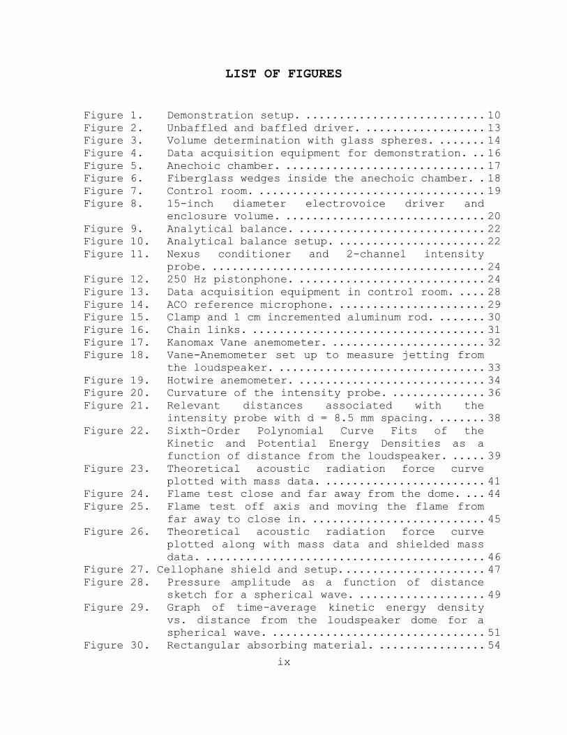
LIST OF FIGURES

Figure 1. Demonstration setup. ........................... 10 Figure 2. Unbaffled and baffled driver. .................. 13 Figure 3. Volume determination with glass spheres. ....... 14 Figure 4. Data acquisition equipment for demonstration. .. 16 Figure 5. Anechoic chamber. .............................. 17 Figure 6. Fiberglass wedges inside the anechoic chamber. . 18 Figure 7. Control room. .................................. 19 Figure 8. 15-inch diameter electrovoice driver and

enclosure volume. .............................. 20 Figure 9. Analytical balance. ............................ 22 Figure 10. Analytical balance setup. ...................... 22 Figure 11. Nexus conditioner and 2-channel intensity

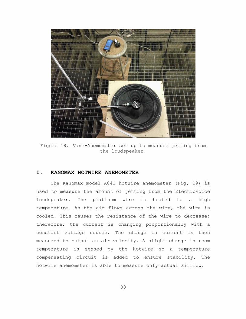
probe. ......................................... 24 Figure 12. 250 Hz pistonphone. ............................ 24 Figure 13. Data acquisition equipment in control room. .... 28 Figure 14. ACO reference microphone. ...................... 29 Figure 15. Clamp and 1 cm incremented aluminum rod. ....... 30 Figure 16. Chain links. ................................... 31 Figure 17. Kanomax Vane anemometer. ....................... 32 Figure 18. Vane-Anemometer set up to measure jetting from

the loudspeaker. ............................... 33 Figure 19. Hotwire anemometer. ............................ 34 Figure 20. Curvature of the intensity probe. .............. 36 Figure 21. Relevant distances associated with the

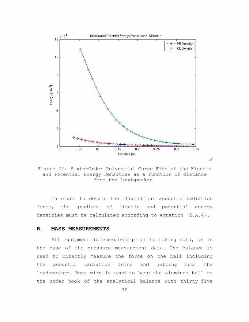
intensity probe with d = 8.5 mm spacing. ....... 38 Figure 22. Sixth-Order Polynomial Curve Fits of the

Kinetic and Potential Energy Densities as a function of distance from the loudspeaker. ..... 39

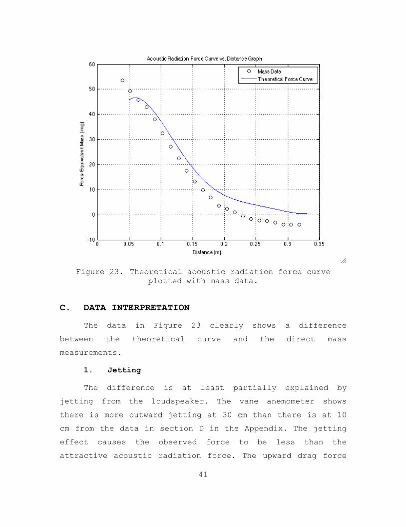
Figure 23. Theoretical acoustic radiation force curve plotted with mass data. ........................ 41

Figure 24. Flame test close and far away from the dome. ... 44 Figure 25. Flame test off axis and moving the flame from

far away to close in. .......................... 45 Figure 26. Theoretical acoustic radiation force curve

plotted along with mass data and shielded mass data. .......................................... 46

Figure 27. Cellophane shield and setup. ..................... 47 Figure 28. Pressure amplitude as a function of distance

sketch for a spherical wave. ................... 49 Figure 29. Graph of time-average kinetic energy density

vs. distance from the loudspeaker dome for a spherical wave. ................................ 51

Figure 30. Rectangular absorbing material. ................ 54

x

Figure 31. Wooden platform supporting the balance and assortment of aluminum bars. ................... 56

Figure 32. Fire suppression system in the anechoic chamber. ....................................... 57

xi

ACKNOWLEDGMENTS

First and foremost, I would like to thank Valerie for

all her support in assisting me through my academics at the

Naval Postgraduate School. Her understanding and endless

love were crucial to my success.

I wish to express my sincere gratitude to Dr. Bruce

Denardo. His vast knowledge and guidance made this research

possible. He has taught me about the difficulties and

complexities of experimental research. His invaluable

mentorship will never be forgotten.

xii


1

I. INTRODUCTION

A. ACOUSTIC RADIATION FORCE AND APPLICATIONS

The acoustic radiation force is a time-averaged force

exerted on a particle by a sound wave. The radiation force

can either be attractive or repulsive depending on the

object’s distance from the acoustic source, wavelength, and

size of the object.

The acoustic attractive portion of the radiation force

due to a traveling wave is thoroughly investigated in this

thesis. The objective is to experimentally verify the

attractive nature of the acoustic radiation force.

There are many applications of the acoustic radiation

force in biology, astrophysics, medicine, and particle

separation. The particle separation research has

significant naval relevance because it is the basis of a

new possible means to remove undesired particles in oil and

to separate oil and water by using ultrasonic methods. The

current method of oil filtration is a centrifuge system

that is antiquated, requires constant attention and is

loud, which is detrimental to stealth on board U.S. Navy

submarines. An acoustic method of filtration would be able

to alleviate many of the previously stated issues, most

notably, loud metallic noises.

B. PREVIOUS WORK

L.V. King (1934) first calculated expressions for the

acoustic radiation force by an incident traveling plane

wave and a standing wave. He used spheres and relatively

long wavelengths in his experiments to test the theory of

2

the acoustic radiation force. T.F.W. Embleton (1951)

continued King’s work by developing a theory and

experimentally testing the acoustic radiation force for

spherical waves by using pendulum deflections. Embleton’s

breakthrough was finding the inverse fifth power

relationship of the force at short distances from a source.

In 1967, W.L. Nyborg (1967) derived a general form for the

acoustic radiation force by assuming the object is located

in the axis of symmetry from the sound field. The result of

his findings is that the force is the difference of the

gradient of the kinetic and potential energy densities,

with a dimensionless factor of the kinetic energy involving

the relative densities of the body and fluid.

Research into various aspects of the acoustic

radiation force has been on-going at the Naval Postgraduate

School since 2004. Stanley Freemyers (2004) attempted to

measure the acoustic radiation force. He used a 15-inch

diameter loudspeaker and varied the voltage amplitude from

5 volts to 40 volts and the frequency from 50 Hz to 200 Hz.

Freemyers’ experimental results showed many deviations from

theory and experimental data; nevertheless, there was very

rough agreement. Spherical wave theory was used, although

this was a poor fit of the sound field.

Michael Schock and Scott Sundem (2005) furthered

Freemyers’ research by observing a significant difference

in an unshielded and shielded acoustic radiation force. A

cellophane “wind shield” was used to enclose the aluminum

sphere to check the acoustic transparency. Their data

indicated an attractive acoustic force on the air.

3

Mario Bentivoglio and James Rochelle (2009)

extensively tested many loudspeaker drivers for acoustic

radiation force measurements. They found the Electrovoice

EVX-155 was best suited for quantitative testing. The

driver was very stable at high amplitudes. Bentivoglio and

Rochelle developed and used a local spherical wave

approximation but had conflicting results between their

experimental data and theory.

Eric Oviatt and Konstantinos Patsiaouras (2009) forced

a spherical wave by placing a 4 foot circular wooden baffle

with a 2.75-inch hole in the center on top of the driver.

They observed strong jetting from the loudspeaker, which

produced an upward drag on the aluminum sphere ball.

Justin Ivanic and Mohamed Akram Zrafi (2011) continued

the work on experimentally verifying the acoustic radiation

force with theory. They used an acoustic intensity probe to

measure the acoustic particle velocity. They found a

systematic error that has not been resolved. Some of the

suspected sources were air currents in the anechoic

chamber, errors in theoretical assumptions, errors in the

theoretical calculation curve, standing wave and

reflections in anechoic chamber and issues with the

accuracy of the intensity probe.

There have been some breakthroughs at the Naval

Postgraduate School but also a number of systematic errors.

This current research is the first to yield reliable

measurements of the acoustic radiation force and to probe

the systematic errors.

The goal of this research is publishable measurements

and predicted values of the acoustic radiation force. The

4

force is measured on an axis of symmetry of the high-

amplitude loudspeaker and measurements of the force on a

small sphere as a function of distance from the source. The

experimental data taken is compared to the theoretical

predictions to determine the extent to which the two agree.

The experiment is be done in the anechoic chamber in

the basement of Spanagel Hall at the Naval Postgraduate

School. The analysis is done in two stages. The first stage

is the experimental calculation of the gradients of kinetic

and potential energies using an intensity probe and a high

amplitude 100 Hz loudspeaker at different ranges. The data

gathered are used to calculate the theoretical radiation

force curve. The second stage involves suspending a solid

aluminum ball suspended from a highly precise analytical

balance at different distances from the loudspeaker. The

acoustic radiation force is measured directly. An analysis

is done comparing the outcome of the two experiments.

5

II. THEORY

A. ACOUSTIC RADIATION FORCE

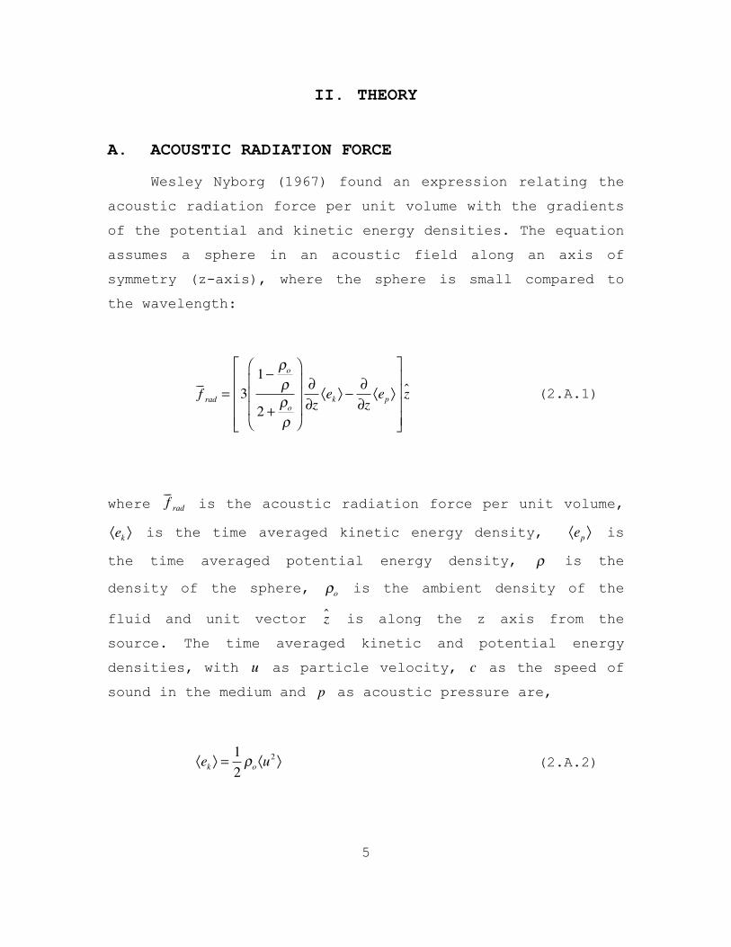
Wesley Nyborg (1967) found an expression relating the

acoustic radiation force per unit volume with the gradients

of the potential and kinetic energy densities. The equation

assumes a sphere in an acoustic field along an axis of

symmetry (z-axis), where the sphere is small compared to

the wavelength:

(2.A.1)

where is the acoustic radiation force per unit volume,

is the time averaged kinetic energy density, is

the time averaged potential energy density, is the

density of the sphere, is the ambient density of the

fluid and unit vector is along the z axis from the

source. The time averaged kinetic and potential energy

densities, with as particle velocity, as the speed of

sound in the medium and as acoustic pressure are,

(2.A.2)

f!"

rad= 3

1!"o"

2 +"o"

#

$

%%%

&

'

(((

))z

*ek + !))z

*ep +

,

-

.

.

.

.

/

0

1111

z#

f!"

rad

!ek" !e

p"

!

!o

z!

u cp

!ek" =

1

2#o!u2 "

6

(2.A.3)

From Nyborg’s expression (2.A.1), the density of air

(1.2 kg/m3) is much less than the density of aluminum (2800

kg/m3) so the approximation ρo/ρAl ≈ 0 can be made in the

equation. The acoustic radiation force equation then

reduces to

(2.A.4)

This equation will be used to test the theory

experimentally.

B. FORCE CAUSED BY A SPHERICAL WAVE ON A BODY

We now consider the acoustic radiation force in the

special case of a traveling spherical wave. Kinsler, Frey,

Coppens and Sanders (2000) express the linear acoustic

pressure and particle velocity of a spherical wave as:

(2.B.1)

(2.B.2)

ep = 12!oc

2 p2 .

f!"rad =

32

!"#

$%&''z

ek ( ''z

ep)*+

,-.z#.

p =A

rcos(!t " kr)

u!= A!ocr

cos("t # kr)+ 1krsin("t # kr)$

%&'()r",

7

where is a constant amplitude, is the frequency and

is the distance from the center of the source.

Substituting equations (2.A.4) and (2.A.5) into

equations (2.A.2) and (2.A.3) yields

(2.B.3)

(2.B.4)

Substituting the kinetic and potential energy

equations (2.A.6) and (2.A.7) respectively into the

acoustic radiation force equation (2.A.1) results in

(2.B.5)

For a spherical wave near a small source kr<<1, the

kinetic energy term then dominates over the potential

energy in equation (2.A.8). The radiation force from a

traveling spherical wave on a small sphere is proportional

to 1/r5.

A ! r

!ek" =

A2

4#oc2r21+

1

kr( )2

$

%&&

'

())

ep = A2

4!oc2r2.

f!"rad = ! 3A2k 3

2"oc2 (kr)5

r#.

8


9

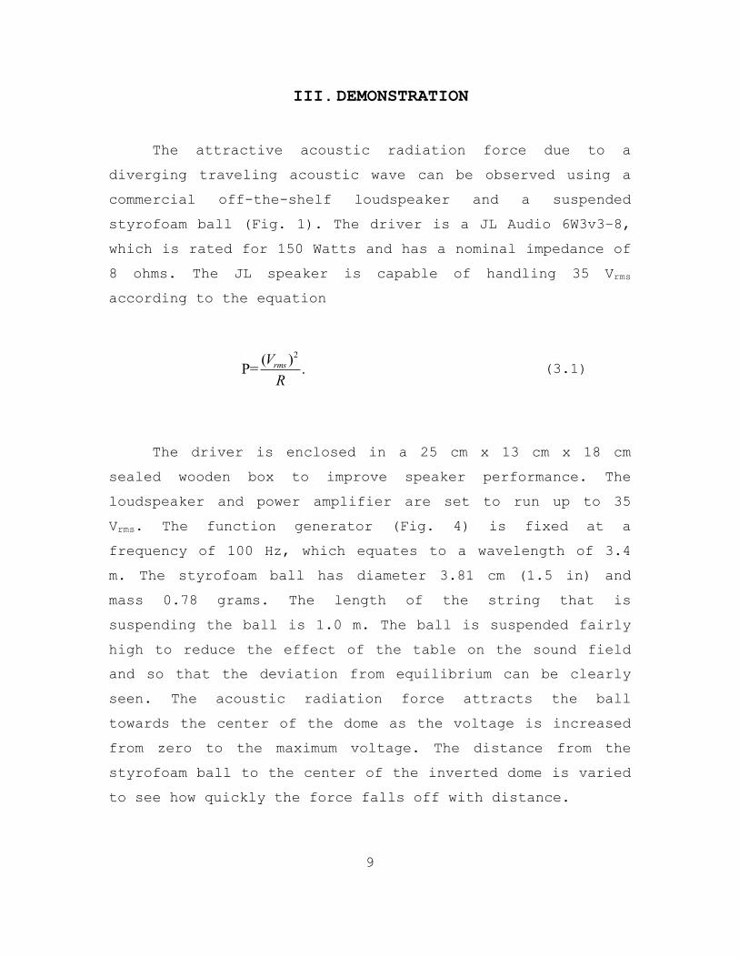
III. DEMONSTRATION

The attractive acoustic radiation force due to a

diverging traveling acoustic wave can be observed using a

commercial off-the-shelf loudspeaker and a suspended

styrofoam ball (Fig. 1). The driver is a JL Audio 6W3v3–8,

which is rated for 150 Watts and has a nominal impedance of

8 ohms. The JL speaker is capable of handling 35 Vrms

according to the equation

2( )P= .rmsVR

(3.1)

The driver is enclosed in a 25 cm x 13 cm x 18 cm

sealed wooden box to improve speaker performance. The

loudspeaker and power amplifier are set to run up to 35

Vrms. The function generator (Fig. 4) is fixed at a

frequency of 100 Hz, which equates to a wavelength of 3.4

m. The styrofoam ball has diameter 3.81 cm (1.5 in) and

mass 0.78 grams. The length of the string that is

suspending the ball is 1.0 m. The ball is suspended fairly

high to reduce the effect of the table on the sound field

and so that the deviation from equilibrium can be clearly

seen. The acoustic radiation force attracts the ball

towards the center of the dome as the voltage is increased

from zero to the maximum voltage. The distance from the

styrofoam ball to the center of the inverted dome is varied

to see how quickly the force falls off with distance.

10

Jetting (Faber, 1995) occurs due to an asymmetry of

pushing a fluid through an orifice as opposed to sucking.

The boundary layer typically quickly separates in the first

case but not in the second. The resultant flow for a

loudspeaker is thus an outward jet. The jetting is more

apparent with a baffled driver and clearly seen using a lit

match or the styrofoam ball. The flame from the lit match

indicates the force due to the jetting. The flame is a

reasonable test to approximate the magnitude of flow at

different distances away from the driver.

Figure 1. Demonstration setup.

11

A. UNBAFFLED DRIVER

The center of the ball is located 10 cm from the

middle of the speaker centered on the inverted dome dust

cover. The ball is suspended close to the driver to

visually see the effects of the acoustic radiation force.

As the voltage is increased from 0 to 35 Vrms, a small

deviation from equilibrium is clearly seen at 15 Vrms and

the styrofoam ball is approximately 7.5 cm from the dome.

As the voltage is increased even further, the ball is

attracted towards the center of the loudspeaker. At 28 Vrms,

there is sufficient force and instability that styrofoam

ball hits the center of the driver which knocks the ball

away. Beyond 10 Vrms, the nonlinearity causes a larger

change in the distance from equilibrium. The acoustic

radiation force is an example of a nonlinear acoustics

effect. The force rapidly decreases as 1/r5 from the source

for a spherical wave.

An unbaffled driver (Fig. 2) forces fluid through the

6-inch diameter speaker so the jetting effects are small.

If a lit match is held a few centimeters away from the

driver at 28 Vrms, the flame is forced outward due to the

loudspeaker’s jetting. Most of the time, the flame is

extinguished by jetting at 2–3 cm from the dome. The

effects of jetting at 10 cm away from the center of the

inverted dome are negligible compared to the acoustic

radiation force.

An approximate value of the acoustic radiation force

can be calculated by using the effective spring constant of

a pendulum using equation (3.A.1). The length ( ) is 1.0 m,

mass ( ) of the styrofoam ball is 0.78 g, gravity ( ) is

L

m g

12

9.8 m/s2 and the observed distance ( ) of the deflected

ball from equilibrium is 2.5 cm. The mass-equivalent

radiation force is about 20 mg. The calculation is shown

below:

(3.A.1)

B. BAFFLED DRIVER

A baffle (Fig. 2) is a plate with a hole in the

center. An acrylic plate is machined to fit over the outer

frame of the driver. The acrylic circular baffle has

diameter of 21.3 cm with a 3 cm diameter hole in the

center. The thickness of the baffle is 1.3 cm. The distance

from the outer edge of faceplate of the baffle to the

center of the inverted dome is 4.5 cm. The baffle causes

more jetting and also more acoustic radiation force due to

a greater acoustic amplitude as a result of the baffle. The

spherical wave solution of the acoustic radiation force is

proportional to the square of the amplitude as seen in

equation (2.B.1).

When the styrofoam ball is placed 10 cm from the

center of the driver, the ball is attracted towards the

driver at 4 Vrms. The acoustic radiation force is clearly

x

Frad = kx

k = mgL

mrad =Fg= mxL

mrad =Fg= mxL

= 0.78g*.025m1m

= 0.0195g ! 20mg

13

much stronger with the baffle. At 14.5 cm from the dome (10

cm from the face of the baffle), jetting dominates and no

acoustic radiation force is observed. When slowing

increasing the voltage to 35 Vrms, the ball is forced away

from the driver at 6.5 Vrms. The jetting significantly

increases due to reducing the size of the orifice from 6 in

bare speaker face (15.24 cm) down to a 3 cm baffle hole.

When a flame is placed at 10 cm or 14.5 cm, the flame is

immediately extinguished when the voltage is increased.

Figure 2. Unbaffled and baffled driver.

1. Helmholtz Resonator

The jetting effect can be increased because the baffle

acts to create a Helmholtz resonator. Using the unflanged

14

effective length equation from KFCS (2000), the resonance

frequency can be calculated from the geometry.

One quantity that is required is the volume of the

baffle-enclosed area (Fig. 3). We found this volume by

using numerous miniscule precision glass spheres to fill

half the area. The spheres are then poured into a graduated

beaker to find the volume. Initially, the baffled area was

completely filled with glass spheres. As more and more

spheres filled the area, the driver cone compressed which

allowed the volume of the baffled area to increase. This

caused the measured volume to be inaccurate. The half

volume filling allows for a more accurate equilibrium

volume calculation.

Figure 3. Volume determination with glass spheres.

15

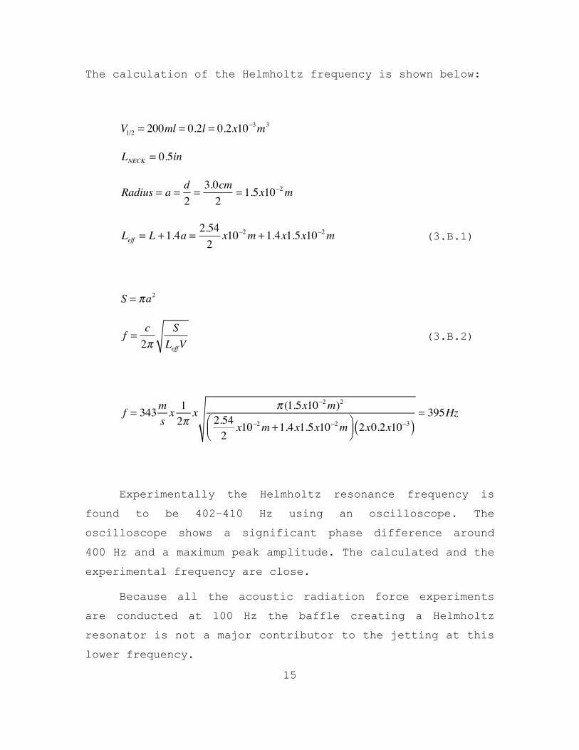
The calculation of the Helmholtz frequency is shown below:

(3.B.1)

(3.B.2)

Experimentally the Helmholtz resonance frequency is

found to be 402–410 Hz using an oscilloscope. The

oscilloscope shows a significant phase difference around

400 Hz and a maximum peak amplitude. The calculated and the

experimental frequency are close.

Because all the acoustic radiation force experiments

are conducted at 100 Hz the baffle creating a Helmholtz

resonator is not a major contributor to the jetting at this

lower frequency.

V1/2 = 200ml = 0.2l = 0.2x10!3m3

LNECK

= 0.5in

Radius = a =d

2=3.0cm

2= 1.5x10

!2m

Leff = L +1.4a =2.54

2x10

!2m +1.4x1.5x10

!2m

S = !a2

f =c

2!

S

LeffV

f = 343msx 12!

x ! (1.5x10"2m)2

2.542

x10"2m +1.4x1.5x10"2m#$%

&'( 2x0.2x10

"3( )= 395Hz

16

Figure 4. Data acquisition equipment for demonstration.

17

IV. EXPERIMENTAL APPARATUS

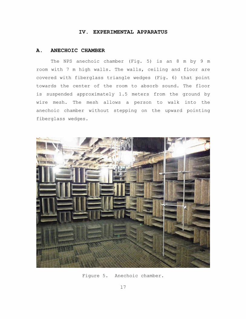
A. ANECHOIC CHAMBER

The NPS anechoic chamber (Fig. 5) is an 8 m by 9 m

room with 7 m high walls. The walls, ceiling and floor are

covered with fiberglass triangle wedges (Fig. 6) that point

towards the center of the room to absorb sound. The floor

is suspended approximately 1.5 meters from the ground by

wire mesh. The mesh allows a person to walk into the

anechoic chamber without stepping on the upward pointing

fiberglass wedges.

Figure 5. Anechoic chamber.

18

The anechoic chamber minimizes traveling wave

reflections produced by a source of sound. The P.F. 612

fiberglass wedges are grouped into three and are

perpendicular to the neighboring group to allow for maximum

absorption.

Figure 6. Fiberglass wedges inside the anechoic chamber.

The control room (Fig. 7) adjacent to the anechoic

chamber is where all the analysis equipment is stored with

the exception of the analytical balance, reference

microphone and conditioner associated with the reference

microphone. The door from the control room into the

anechoic chamber is also lined with the same fiberglass

19

material to ensure uniformity. There are small window ports

to allow cables into and out of the chamber.

Figure 7. Control room.

20

B. DRIVER ASSEMBLY

The loudspeaker (Fig. 8) is a 15-inch diameter

Electro-Voice EVX-155 that has been re-coned at Santa Cruz

Sound Company in Santa Cruz, Ca. The power handling

capability is 600 W (continuous) and the nominal impedance

is 8 ohms.

The driver is contained in a 0.46 m x 0.46 m x 0.56 m

wooden enclosure. The speaker and enclosure are oriented

vertically so that the sound field travels upward towards

the analytic balance. This allows the aluminum sphere to

hang symmetrically above the peak of the cone. The driver’s

wooden enclosure is on a platform built to hold the driver

just above the wire mesh of the anechoic chamber.

Figure 8. 15-inch diameter electrovoice driver and enclosure volume.

21

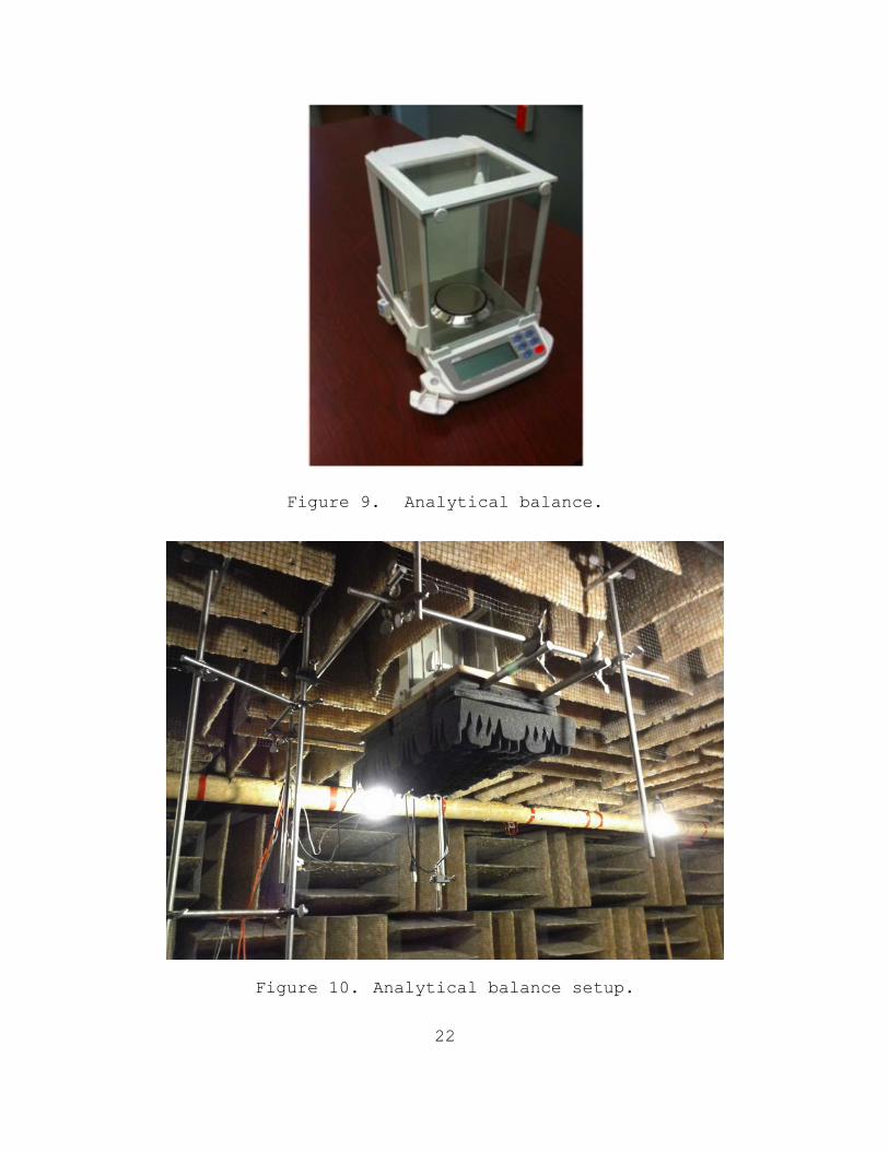
C. ANALYTICAL BALANCE

The high precision balance (Fig. 9) is an AND GR-202

Analytical Balance. The AND balance has a built-in hook

underneath the balance to allow for precision measurements

to be made outside the weighing chamber. A hook holds the

aluminum sphere. The acoustic radiation force (F ) due to the loudspeaker can be easily calculated from the mass

reading (m ) of the balance as F mg= , where g is the

acceleration due to gravity. There is a secondary display

and a push button to zero the balance in the control room.

An operator does not have to physically stand in the

anechoic chamber while gathering measurements (Fig.10). The

specifications of the balance are as follows:

SPECIFICATIONS

Weighting Capacity 210 g/42 g

Min. weighing value (1 digit) 0.1 mg/0.01 mg

Repeatability (Std dev) 0.1 mg/0.02 mg

Stabilization time 3.5 sec/ 8 sec

Calibration weight Built-in

Net weight Approx. 6.0 kg

22

Figure 9. Analytical balance.

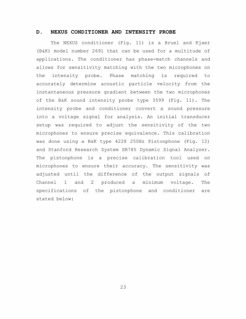
Figure 10. Analytical balance setup.

23

D. NEXUS CONDITIONER AND INTENSITY PROBE

The NEXUS conditioner (Fig. 11) is a Bruel and Kjaer

(B&K) model number 2691 that can be used for a multitude of

applications. The conditioner has phase-match channels and

allows for sensitivity matching with the two microphones on

the intensity probe. Phase matching is required to

accurately determine acoustic particle velocity from the

instantaneous pressure gradient between the two microphones

of the B&K sound intensity probe type 3599 (Fig. 11). The

intensity probe and conditioner convert a sound pressure

into a voltage signal for analysis. An initial transducer

setup was required to adjust the sensitivity of the two

microphones to ensure precise equivalence. This calibration

was done using a B&K type 4228 250Hz Pistonphone (Fig. 12)

and Stanford Research System SR785 Dynamic Signal Analyzer.

The pistonphone is a precise calibration tool used on

microphones to ensure their accuracy. The sensitivity was

adjusted until the difference of the output signals of

Channel 1 and 2 produced a minimum voltage. The

specifications of the pistonphone and conditioner are

stated below:

24

Figure 11. Nexus conditioner and 2-channel intensity probe.

Figure 12. 250 Hz pistonphone.

25

PISTONPHONE

Sound Pressure Level 124.08 re 20uPa

Nominal Frequency 250Hz +/- 0.1%

Calibrated 25 APR 2011

NEXUS CONDITIONER SETUP

Amplifier Setup

CH 1/CH 2 3.16mV/Pa / 3.16mV/Pa

Transducer Setup Sensitivity

CH 1/CH 2 11.933mV/Pa / 11.967mV/Pa

Transducer Supply

Supply Voltage Polarization Cable length

CH 1 14V 200V 8m

CH 2 14V 200V 8m

NOTE: Channel 1 is Channel A

Channel 2 is Channel B

E. ELECTRONIC DATA ACQUISITION EQUIPMENT AND SETUP

Most of the electrical equipment (Fig. 13) required

for the experiment was inside the anechoic chamber control

room. The driving circuit has an HP 33120a function

generator and a QSC MX3000a Dual Monaural Amplifier. The

two-channel intensity probe signals are fed into the B&K

NEXUS conditioner and then into the Stanford Research

26

System SR560 Low Noise Preamplifier. The amplified signal

is sent to Stanford FFT Spectrum Analyzer to obtain voltage

output data.

The Stanford preamp is able to take both channels and

to output Channel A, Channel B or more importantly the

difference between the two channels. The difference output

gives the instantaneous pressure difference between Channel

A and B from the intensity probe. The FFT analyzer is able

to isolate the voltage output signal.

An ACO half-inch microphone (Fig. 14), which serves as

a reference microphone is connected to a HP34401A digital

multimeter and is located about 1 meter above and to one

side the driver. To ensure accuracy and consistency in the

data, the reference microphone voltage is held constant as

the height of the intensity probe and aluminum ball varies.

The reference microphone output voltage is seen on the

multimeter, which is located in the control room.

The balance has a remote display with zeroing

capability inside the control room. This allows for

streamlining data taking process because the analytical

balance is suspended on a platform attached to the ceiling

of the anechoic chamber. A stool must be used to locally

read the scale in the anechoic chamber. The specifications

of the preamplifier and microphone are shown below:

27

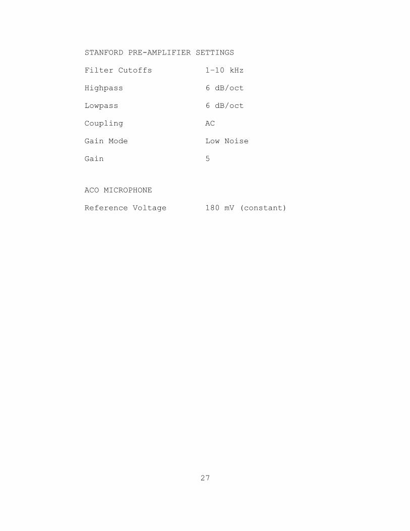
STANFORD PRE-AMPLIFIER SETTINGS

Filter Cutoffs 1–10 kHz

Highpass 6 dB/oct

Lowpass 6 dB/oct

Coupling AC

Gain Mode Low Noise

Gain 5

ACO MICROPHONE

Reference Voltage 180 mV (constant)

28

Figure 13. Data acquisition equipment in control room.

29

Figure 14. ACO reference microphone.

F. ALUMINUM ROD AND INTENSITY PROBE CLAMP

A 1/2-inch diameter 8-ft long aluminum rod (Fig. 15)

was machined with forty grooves that were ink-marked. The

grooves are in 1 cm increments from one end of the rod.

This alleviated the ambiguity in measuring the exact

distance from the peak of the cone in the center of the

driver. The markings sped up data taking when many distance

measurements were required. The only measurement that

required a ruler was the initial distance from the center

of the cone to the closest microphone on the intensity

30

probe. Every groove has a mark with permanent black ink

with the exception of every fifth one which is delineated

with red.

The intensity probe clamp (Fig. 15) was machined to

allow the probe to be raised in 1 cm increments. The clamp

has a small thin brass plate, which fits inside the grooves

of the aluminum rod. A plastic insert was also placed on

the end of the screw clamp to prevent scoring of the

intensity probe extender rod.

Figure 15. Clamp and 1 cm incremented aluminum rod.

31

G. CHAIN LINK SPACERS AND BUSS WIRE

For ease of data collection and reproduction,

individual chain links (Fig. 16) were cut from a single

steel chain to obtain nearly exact distances. Several

different mathematical methods of individual link

calculations were used to obtain the distance. The

calculated distance is 1.2655 cm of each link. Twenty links

is sufficient to obtain the acoustic radiation force

measurements. The aluminum sphere distance to the

loudspeaker dome is incremented 1.2655 cm at a time to

obtain the force on axis of the loudspeaker.

Thirty-two gauge buss wire connects the aluminum

sphere to the chain link spacer. Buss wire allows the ball,

wire and chain to be electrically grounded to ensure there

are no electrostatic effects.

Figure 16. Chain links.

32

H. KANOMAX VANE ANEMOMETER

The Kanomax model 6812 volume flow anemometer (Fig.

17) is used to measure the amount of jetting from the

Electrovoice loudspeaker. The anemometer uses an extremely

low friction vane-type probe to measure the flow rate

through the vane in meters per second. The flow rate in

meters per second can be used to calculate into milligrams

of drag force to account for the jetting (Fig. 18). The

specifications of the anemometer are as follows:

SPECIFICATIONS

Propeller Vane Diameter 70 mm

Sensitivity 0.20–40.00 m/s

Sampling Rate 2 sec

Figure 17. Kanomax Vane anemometer.

33

Figure 18. Vane-Anemometer set up to measure jetting from the loudspeaker.

I. KANOMAX HOTWIRE ANEMOMETER

The Kanomax model A041 hotwire anemometer (Fig. 19) is

used to measure the amount of jetting from the Electrovoice

loudspeaker. The platinum wire is heated to a high

temperature. As the air flows across the wire, the wire is

cooled. This causes the resistance of the wire to decrease;

therefore, the current is changing proportionally with a

constant voltage source. The change in current is then

measured to output an air velocity. A slight change in room

temperature is sensed by the hotwire so a temperature

compensating circuit is added to ensure stability. The

hotwire anemometer is able to measure only actual airflow.

34

Figure 19. Hotwire anemometer.

35

V. EXPERIMENT

The experiment is divided into two distinct phases.

The first phase is obtaining the theoretical prediction

curve by taking pressure measurements of the acoustic

field. The pressure measurements are used to find the

gradient of the kinetic and potential energy densities

resulting in the acoustic radiation force. The second phase

is taking actual mass-equivalent force measurements to

compare with the theoretical prediction.

A. PRESSURE MEASUREMENTS

The pressure measurements are taken first to obtain

the theoretical acoustic radiation force curve. All the

analyzing equipment is energized an hour and a half prior

to taking data to establish thermodynamic equilibrium. Due

to the curvature of the bottom of the intensity probe (Fig.

20), the lower microphone (“A”) is placed 3.6 cm above the

dome of the loudspeaker. This is the closest distance

without the loudspeaker dome contacting the bottom of the

probe as the dome oscillates. As the voltage of the driver

is increased to approximately 60 VAC, the reference

microphone input voltage is adjusted to maintain 180 mV to

ensure a constant acoustic field and reproducibility. When

the voltage is stable at 180 mV at approximately 30

seconds, microphone A rms voltage and Stanford pre-

amplifier A–B rms voltage is taken using the FFT spectrum

analyzer, which is set up to read the voltage amplitude at

100 Hz. After the two voltages are recorded, the driver is

turned off and the intensity probe distance is increased by

one centimeter from the driver on the aluminum rod.

36

Figure 20. Curvature of the intensity probe.

A five-minute wait on the stopclock is started to

allow for the driver to return to equilibrium. After the

five-minute wait, the driver voltage is increased to

approximately 60 VAC and the reference microphone is

maintained at 180 mV then the second voltage data points

are taken. This data-taking process is repeated thirty

times to ensure there are enough data points to fit a

curve.

The voltages in section A of the Appendix are

converted into pressures by using 3.16 mV/Pa conversion

factor displayed on the Nexus conditioner. The gain from

the Stanford pre-amplifier is divided out. The kinetic

energy density uses the linearized Euler’s equation for the

amplitude of the particle velocity

37

(5.A.1)

where is the frequency of 100 Hz, is the density of

air, =8.5 mm is the distance between the two microphone

membranes and is the amplitude of the instantaneous

difference in the pressures of microphones A and B. The

particle velocity amplitude is then used to calculate the

kinetic energy density (2.A.2) and the potential energy

density (2.A.3). The results of the calculations are in

section B of the Appendix.

The distance calculations for the KE and PE densities

for the intensity probe are located in Figure 21. The

gathered data from section B is plotted in Matlab. A curve

fit tool in Matlab fits the data points using a sixth order

polynomial. The curve fits are shown in Figure 22.

U=Pdiff

2! f "d,

f !

d

Pdiff

38

Figure 21. Relevant distances associated with the intensity probe with d = 8.5 mm spacing.

39

Figure 22. Sixth-Order Polynomial Curve Fits of the Kinetic and Potential Energy Densities as a function of distance

from the loudspeaker.

In order to obtain the theoretical acoustic radiation

force, the gradient of kinetic and potential energy

densities must be calculated according to equation (2.A.4).

B. MASS MEASUREMENTS

All equipment is energized prior to taking data, as in

the case of the pressure measurement data. The balance is

used to directly measure the force on the ball including

the acoustic radiation force and jetting from the

loudspeaker. Buss wire is used to hang the aluminum ball to

the under hook of the analytical balance with thirty-five

40

chain links in between. The initial ball height from the

dome is 2.07 cm with an added 1.905 cm (radius of the ball)

for a total of 3.98 cm.

The voltage is increased on the driver to

approximately 60 VAC at 100 Hz. The reference microphone is

maintained at 180 mV. When the balance reading is steady in

approximately 30 seconds, the balance reading is read off

the remote display in the control room. After the balance

weight is taken, the loudspeaker is turned off. The

anechoic chamber is entered to remove a single link off the

chain. A five-minute wait on the stopclock is started to

allow for equilibrium.

After the five-minute wait, this process is repeated

twenty-three times to give a final distance of 33.08 cm

(1.2655 cm x 23 links + 3.975 cm). The final mass data is

located in section C of the Appendix. Figure 23 shows the

plot of the final mass data with the theoretical curve.

41

Figure 23. Theoretical acoustic radiation force curve

plotted with mass data.

C. DATA INTERPRETATION

The data in Figure 23 clearly shows a difference

between the theoretical curve and the direct mass

measurements.

1. Jetting

The difference is at least partially explained by

jetting from the loudspeaker. The vane anemometer shows

there is more outward jetting at 30 cm than there is at 10

cm from the data in section D in the Appendix. The jetting

effect causes the observed force to be less than the

attractive acoustic radiation force. The upward drag force

42

on the ball can be calculated. Cengel and Cimbala (2010)

give the general drag force equation as

(5.C.1)

where is the density of air of 1.204 kg/m3, is the

cross-sectional area, is the velocity and is the

drag coefficient of the volume associated with a specific

Reynolds number R . The Reynolds number for a sphere is

(5.C.2)

where is the diameter and is the kinematic viscosity of

air at room temperature and atmospheric pressure. At a

distance of 0.30 m from the loudspeaker dome the vane

anemometer reads 0.33 m/s, so

( ) 5 2

m 0.0254R=U 0.33 * 1.5 * * 838.1.516 10

d m sinv s in x m−

⎛ ⎞ ⎛ ⎞ ⎛ ⎞= =⎜ ⎟ ⎜ ⎟ ⎜ ⎟⎝ ⎠ ⎝ ⎠ ⎝ ⎠

A Reynolds number of 838 yields a drag coefficient of

approximately 0.6 from the CD vs. Reynolds number graph from

Cengel and Cimbala(2010). The drag force is then

FD = 12!oU

2SCD (R),

!o S

U CD (R)

R=U dv,

d v

43

25

2

3

1 1.204 0.33 0.0254* * * * 0.75 * *0. 4.48 10 ,62D

kg m mF inm s in

x Nπ −⎛ ⎞⎛ ⎞ ⎛ ⎞ ⎛ ⎞= =⎜ ⎟ ⎜ ⎟ ⎜ ⎟⎜ ⎟⎝ ⎠ ⎝ ⎠ ⎝ ⎠⎝ ⎠

6 21 10 * 4.574 .9.8

DF x mg s mgg kg m

⎛ ⎞ ⎛ ⎞= =⎜ ⎟ ⎜ ⎟⎝ ⎠ ⎝ ⎠

The calculated drag force of 4.6 mg accounts for 70%

of the difference between the direct force-mass measurement

and the theoretical curve. The points for the mass data

should be higher and closer to the theoretical curve. The

vane anemometer is averaging over a wider area of due to

the diameter of the vane being 6.98 cm (2.75 in) while the

ball is 3.81 cm (1.5 in). The difference in area could

cause the deviation from theory to actual data. This

discrepancy requires further research.

A hotwire anemometer is also used to find the airflow

rate of the jetting. The wire of the hotwire anemometer is

a much smaller sensor than the vane anemometer. The hotwire

is able to output a more localized airflow reading. The

hotwire anemometer senses a higher jetting flow rate

approaching the dome shown in section D of the Appendix,

which is contradictory to the vane anemometer. The two

anemometers approximately agree at 30 cm but deviate closer

in.

Since the vane anemometer is averaging over a larger

area, we conclude the jetting is very turbulent near the

dome. The vane anemometer is reading both upward and

downward flow to cause cancellations approximating zero.

44

Unfortunately, the hotwire anemometer is not able to output

flow direction so an inward flow towards the driver could

not be measured.

Since the fluid dynamics around the dome of the driver

is so complex, the jetting force and direction is crudely

measured by using a flame (Fig. 24). A lit match is able to

check the relative jetting force, as the flame is taken

closer to the dome. In theory, the direction of the flame

on and off axis can also be roughly seen (Fig. 25). The

flame is erratic on and off axis near the dome. The result

of these tests proves to be inconclusive.

Figure 24. Flame test close and far away from the dome.

45

Figure 25. Flame test off axis and moving the flame from far away to close in.

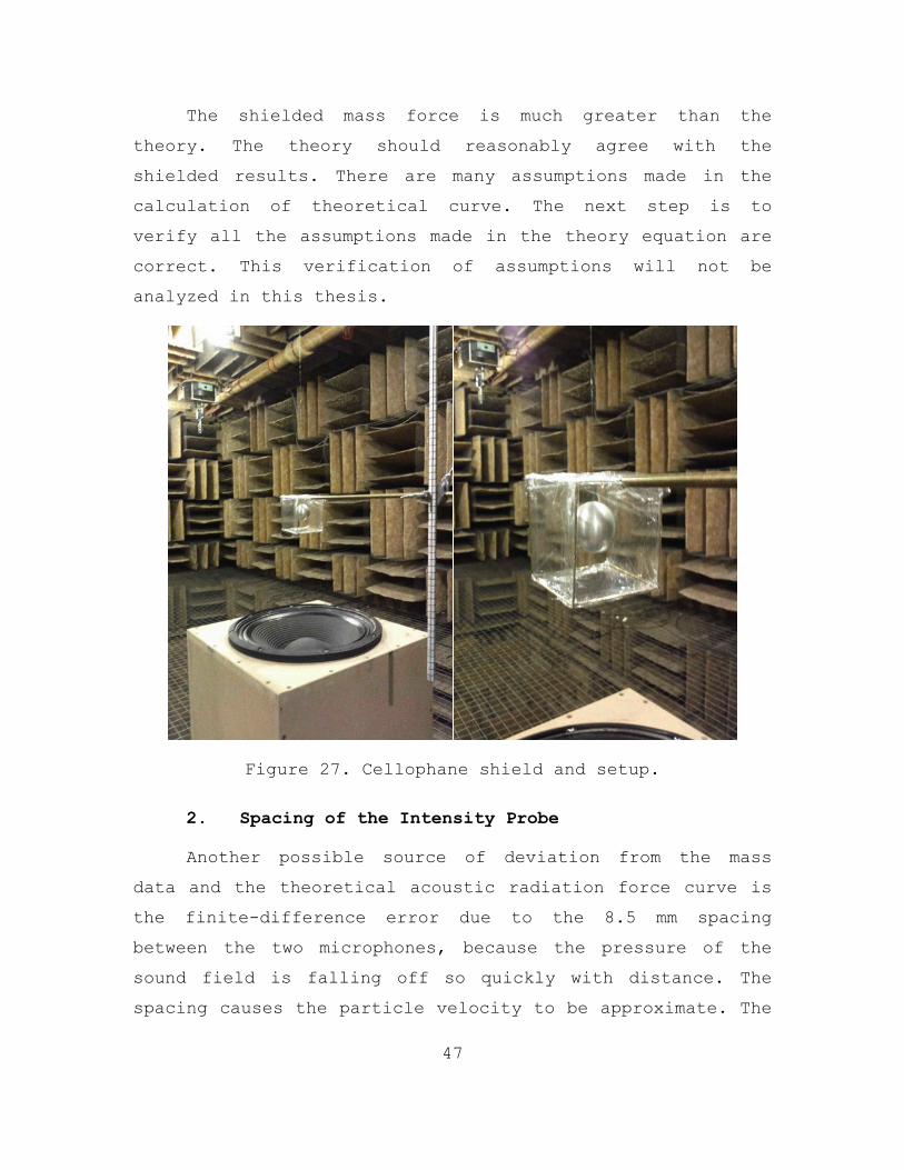
In attempt to nullify the amount of jetting around the

ball, a cubical cellophane shield was created (Fig. 27).

The cube is 3.0 inches on a side with a hole at the top to

just allow for the 3.81 cm (1.5 in) diameter aluminum ball

to enter. A mass measurement is taken at 30 cm from the top

of the dome with and without the cube. Without the cube,

the analytic balance measures negative 4.4 mg, which is

consistent with the previous mass data. With the cube, the

analytic balance measures a positive 1.6 mg at 30 cm from

the dome shown in section E of the Appendix. The theory

line at 30 cm is 1.4 mg. There is agreement between theory

and shielded mass data. The cube is able to divert most of

the jetting flow around the aluminum ball.

At 7 cm, there is another discrepancy from the

original mass data (Fig. 26). Surprisingly, the mass

46

reading with the shield is 230 mg, whereas the mass reading

without the shield is 45.7 mg. The difference in mass at 7

cm is approximately 184 mg. Using the drag force equation

(5.C.1) and a velocity of 1.6 m/s, only 109 mg is accounted

for due to jetting. The drag force equation assumes a

laminar steady flow. The flow is very turbulent near the

source. Some of the mass equivalent force of 75 mg could be

due to turbulent flow but that is only a speculation. The

discrepancy is unknown and requires further investigation.

Figure 26. Theoretical acoustic radiation force curve plotted along with mass data and shielded mass data.

47

The shielded mass force is much greater than the

theory. The theory should reasonably agree with the

shielded results. There are many assumptions made in the

calculation of theoretical curve. The next step is to

verify all the assumptions made in the theory equation are

correct. This verification of assumptions will not be

analyzed in this thesis.

Figure 27. Cellophane shield and setup.

2. Spacing of the Intensity Probe

Another possible source of deviation from the mass

data and the theoretical acoustic radiation force curve is

the finite-difference error due to the 8.5 mm spacing

between the two microphones, because the pressure of the

sound field is falling off so quickly with distance. The

spacing causes the particle velocity to be approximate. The

48

spherical wave fit of the pressure amplitude is used to

verify if the finite spacing is a source of error:

,APx b

=+

(5.C.3)

where, in SI units, x is the distance from dome, A = 24.44 and b = 0.04771 by using a curve-fit tool software. The

peak amplitudes of the gradients are determined by

instantaneous pressure between x0 and x0±d (Fig. 28). From

the gradient values, the velocity amplitudes are determined

and then the average kinetic energy densities. These

average kinetic energy density values are plotted against

the exact theoretical curve for the average kinetic energy

of a spherical wave. The error between the two is analyzed.

The instantaneous pressure at x0 using equation (2.B.1)

is

[ ]0 00

cos ( ) .Ap k x b tx b

ω= + −+

(5.C.4)

49

Figure 28. Pressure amplitude as a function of distance sketch for a spherical wave.

The instantaneous pressure at x0±d using equation

(2.B.1) is

[ ]00

cos ( ) .Ap k x d b tx d b

ω± = ± + −± +

(5.C.5)

The instantaneous gradients of the pair of points are then

[ ] [ ]0 0

0 0

cos ( ) cos ( ).

k x d b t k x b tApd x d b x b

ω ω±

⎧ ⎫± + − + −∇ = −⎨ ⎬± + +⎩ ⎭

(5.C.6)

50

The peak particle velocity amplitudes can be found from the

Euler-equation relationship

,2p

Ufπ ρ±

±

∇= (5.C.7)

where f is 100 Hz and ! is 1.204 kg/m3 for the density of

air. The time-averaged kinetic energy densities are

2

.4kUe ρ ±

±= (5.C.8)

The exact instantaneous particle velocity for a spherical

wave is equation (2.B.2). The exact time-averaged kinetic

energy density is

2

2 2 2 2

11 .4kAec r k rρ

⎛ ⎞= +⎜ ⎟⎝ ⎠ (5.C.9)

The curves ke and ke ± vs. x are plotted on the same

curve to determine the error (Fig. 29). The curve is exact

and the points correspond to a finite-difference

approximation that is used for the intensity probe. There

is very little error caused by the 8.5 mm spacer on the

intensity probe. This is not a source of error in our

experiment.

51

Figure 29. Graph of time-average kinetic energy density vs. distance from the loudspeaker dome for a spherical wave.

3. Data Approaching Zero

The mass data curve in the tail should go to zero as

in the theory. The mass data does approach zero but at much

farther distance, as shown in section F of the Appendix. At

125 cm, the analytical balance reads nearly zero.

0.05 0.10 0.15 0.20 0.25 0.30 0.350

1

2

3

4

5

time-

aver

aged

kin

etic

ene

rgy

dens

ity <

e k> (J

/m3 )

distance from dome x (m)

52


53

VI. CONCLUSION

There is approximate agreement between the calculated

theory curve and the directly measured mass data shown in

Figure 23. The disparity comes with the shielded cube data

and the theory. The source of the disagreement requires

further research.

Many issues exist in the experiment such as:

complexity in fluid dynamics near the dome, finite-size

effects and thermoviscous losses. There are other minor

issues, which could possibly contribute to the deviation

between theory and experiment. Some of these are explained

below.

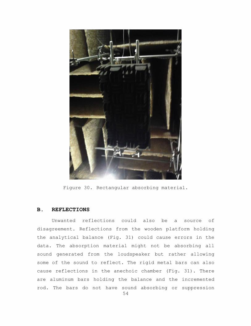
A. AXIS OF SYMMETRY

One source of deviation could be due to the lack of

symmetry. The driver’s enclosure is a wooden box that has

four distinct corners instead of a circular base. The

theory states an axis of symmetry must be preserved. The

absorption material below the balance platform is also

rectangular (Fig. 30). The theory states that symmetry is

crucial to the experiment. An extensive and careful probing

of the acoustic field off-axis would establish the degree

to which the field is symmetric about the axis. Quick

measurements show only at most a 1% asymmetry of the field

over the diameter of the sphere, so a lack of symmetry of

the field does not appear to be playing a role.

54

Figure 30. Rectangular absorbing material.

B. REFLECTIONS

Unwanted reflections could also be a source of

disagreement. Reflections from the wooden platform holding

the analytical balance (Fig. 31) could cause errors in the

data. The absorption material might not be absorbing all

sound generated from the loudspeaker but rather allowing

some of the sound to reflect. The rigid metal bars can also

cause reflections in the anechoic chamber (Fig. 31). There

are aluminum bars holding the balance and the incremented

rod. The bars do not have sound absorbing or suppression

55

materials on or around them. A new fire extinguishing

system was installed in the anechoic chamber at the Naval

Postgraduate School in 2010 (Fig. 32). The piping is not

insulated by sound. The metal piping lining the left side

of the anechoic chamber could be also causing reflections.

The reflections would cause errors in both the mass and

pressure data.

It should be noted that reflections themselves do not

invalidate the theory, which is valid even for standing

waves (Nyborg, 1967). However, reflections here would

probably degrade the symmetry of the acoustic field about

the axis (sec. A), which violates the theory.

56

Figure 31. Wooden platform supporting the balance and assortment of aluminum bars.

57

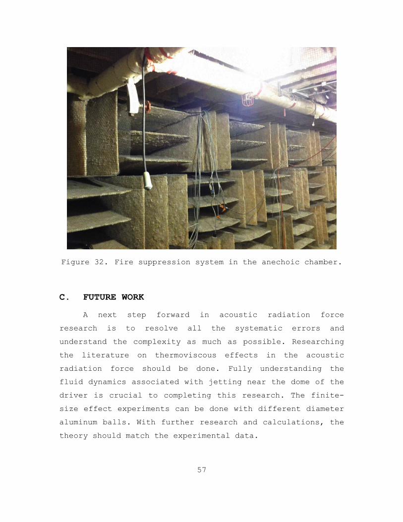
Figure 32. Fire suppression system in the anechoic chamber.

C. FUTURE WORK

A next step forward in acoustic radiation force

research is to resolve all the systematic errors and

understand the complexity as much as possible. Researching

the literature on thermoviscous effects in the acoustic

radiation force should be done. Fully understanding the

fluid dynamics associated with jetting near the dome of the

driver is crucial to completing this research. The finite-

size effect experiments can be done with different diameter

aluminum balls. With further research and calculations, the

theory should match the experimental data.

58

However, we have shown approximate agreement between

theory and experiment, which allows us to move forward to

performing ultrasonic filtration experiments. The first

step is a simple proof-of-principle experiment with

neutrally-buoyant particles in water, which would bring us

one step closer to actual shipboard application of the

acoustic radiation force phenomena.

59

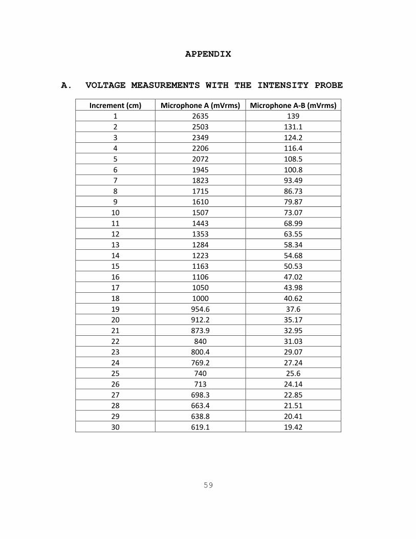
APPENDIX

A. VOLTAGE MEASUREMENTS WITH THE INTENSITY PROBE

Increment (cm) Microphone A (mVrms) Microphone A-‐B (mVrms) 1 2635 139 2 2503 131.1 3 2349 124.2 4 2206 116.4 5 2072 108.5 6 1945 100.8 7 1823 93.49 8 1715 86.73 9 1610 79.87 10 1507 73.07 11 1443 68.99 12 1353 63.55 13 1284 58.34 14 1223 54.68 15 1163 50.53 16 1106 47.02 17 1050 43.98 18 1000 40.62 19 954.6 37.6 20 912.2 35.17 21 873.9 32.95 22 840 31.03 23 800.4 29.07 24 769.2 27.24 25 740 25.6 26 713 24.14 27 698.3 22.85 28 663.4 21.51 29 638.8 20.41 30 619.1 19.42

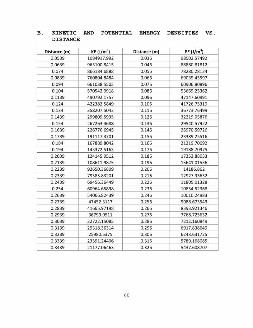
60

B. KINETIC AND POTENTIAL ENERGY DENSITIES VS. DISTANCE

Distance (m) KE (J/m3) Distance (m) PE (J/m3) 0.0539 1084917.992 0.036 98502.57492 0.0639 965100.8415 0.046 88880.81812 0.074 866184.6888 0.056 78280.28134 0.0839 760804.8484 0.066 69039.45597 0.094 661038.5503 0.076 60906.80896 0.104 570542.9918 0.086 53669.25362 0.1139 490792.1757 0.096 47147.60991 0.124 422382.5849 0.106 41726.75319 0.134 358207.5042 0.116 36773.76499 0.1439 299809.5935 0.126 32219.05876 0.154 267263.4688 0.136 29540.57922 0.1639 226776.6945 0.146 25970.59726 0.1739 191117.3701 0.156 23389.25516 0.184 167889.8042 0.166 21219.70092 0.194 143372.5163 0.176 19188.70975 0.2039 124145.9512 0.186 17353.88033 0.2139 108611.9875 0.196 15641.01536 0.2239 92650.36809 0.206 14186.862 0.2339 79385.83201 0.216 12927.93632 0.2439 69456.36449 0.226 11805.01328 0.254 60964.65898 0.236 10834.52368 0.2639 54066.82439 0.246 10010.24983 0.2739 47452.3117 0.256 9088.673543 0.2839 41665.97198 0.266 8393.921346 0.2939 36799.9511 0.276 7768.725632 0.3039 32722.15085 0.286 7212.160849 0.3139 29318.36314 0.296 6917.838649 0.3239 25980.5375 0.306 6243.631725 0.3339 23391.24406 0.316 5789.168085 0.3439 21177.06463 0.326 5437.608707

61

C. MASS DATA FROM THE ANALYTICAL BALANCE

Link distances (m) Mass (mg) 0.03975 53.5 0.052405 49.2 0.06506 45.7 0.077715 42.9 0.09037 37.9 0.103025 32.4 0.11568 27.2 0.128335 22.4 0.14099 17.5 0.153645 13.3 0.1663 9.8 0.178955 6.9 0.19161 3.7 0.204265 2.3 0.21692 0.9 0.229575 -‐0.7 0.24223 -‐1.8 0.254885 -‐2.3 0.26754 -‐2.5 0.280195 -‐3.1 0.29285 -‐4 0.305505 -‐4 0.31816 -‐4

D. HOTWIRE AND VANE ANEMOMETER READINGS

Distance (cm) Vane Anemometer (m/s) Hotwire Anemometer (m/s) 30 0.3 0.33 25 0.31 Not Taken 20 0.31 0.35 15 0.26 0.66 10 0 1.18 6 0 1.61

62

E. MASS READINGS WITH CELLOPHANE SHIELD

Distance (cm) Mass w/ shield (mg) 30 1.7 25 4.6 20 10.9 15 35.4 10 96.7 7 230

F. ROUGH MASS READINGS AT FURTHER DISTANCES

Distance (cm) Mass (mg) 50 -‐4.4 75 -‐2.9 100 -‐2 125 -‐1

G. MATLAB CODE

clc; clear; %voltages A = [2635;2503;2349;2206;2072;1945;1823;1715;1610;1507;1443;1353;1284;1223;1163;1106;1050;1000;954.6;912.2;873.9;840;800.4;769.2;740.0;713;698.3;663.4;638.8;619.1]; AminusB=[139;131.1;124.2;116.4;108.5;100.8;93.49;86.73;79.87;73.07;68.99;63.55;58.34;54.68;50.53;47.02;43.98;40.62;37.6;35.17;32.95;31.03;29.07;27.24;25.6;24.14;22.85;21.51;20.41;19.42]; %distance meters 30 points zAm=[0.036:0.01:0.3260]; %middle of mic 0.036m+0.01795 m=0.05395m to 0.34395 (8.5mm spacer) zAminusBm=[0.05395:0.01:0.34395]; %pressure conversion P_A=A./3.16e-3./5; P_AminusB=AminusB./3.16e-3./5; figure (1) hold on; %plot of A

63

plot(zAm,A,’-.*r’) %plot of A minus B plot(zAminusBm,AminusB,’:og’) %PE PEz=P_A.^2./(2*1.2*343^2); %KE U=P_AminusB./(2*pi*100*1.225*.0085); % 8.5mm spacer KEz=0.5.*(1.2.*U.^2); %cftool % % Linear model Poly6: % f(x) = p1*x^6 + p2*x^5 + p3*x^4 + p4*x^3 + p5*x^2 + % p6*x + p7 % Coefficients (with 95% confidence bounds): % p1 = -1.052e+09 (-1.477e+09, -6.267e+08) % p2 = 1.175e+09 (7.12e+08, 1.638e+09) % p3 = -4.96e+08 (-6.942e+08, -2.978e+08) % p4 = 9.121e+07 (4.899e+07, 1.334e+08) % p5 = -3.756e+06 (-8.412e+06, 8.995e+05) % p6 = -1.095e+06 (-1.342e+06, -8.474e+05) % p7 = 1.397e+05 (1.348e+05, 1.445e+05) % % Goodness of fit: % SSE: 1.261e+06 % R-square: 0.9999 % Adjusted R-square: 0.9999 % RMSE: 234.1 % % % Linear model Poly6: % f(x) = p1*x^6 + p2*x^5 + p3*x^4 + p4*x^3 + p5*x^2 + % p6*x + p7 % Coefficients (with 95% confidence bounds): % p1 = -1.421e+10 (-1.943e+10, -8.991e+09) % p2 = 1.85e+10 (1.226e+10, 2.474e+10) % p3 = -9.456e+09 (-1.242e+10, -6.492e+09) % p4 = 2.324e+09 (1.614e+09, 3.035e+09) % p5 = -2.489e+08 (-3.388e+08, -1.59e+08) % p6 = 6.729e+05 (-4.956e+06, 6.302e+06) % p7 = 1.478e+06 (1.343e+06, 1.613e+06) % % Goodness of fit: % SSE: 1.897e+08 % R-square: 0.9999 % Adjusted R-square: 0.9999 % RMSE: 2872

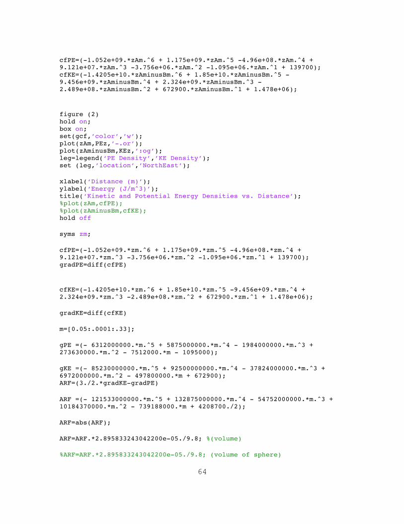
64

cfPE=(-1.052e+09.*zAm.^6 + 1.175e+09.*zAm.^5 -4.96e+08.*zAm.^4 + 9.121e+07.*zAm.^3 -3.756e+06.*zAm.^2 -1.095e+06.*zAm.^1 + 139700); cfKE=(-1.4205e+10.*zAminusBm.^6 + 1.85e+10.*zAminusBm.^5 -9.456e+09.*zAminusBm.^4 + 2.324e+09.*zAminusBm.^3 -2.489e+08.*zAminusBm.^2 + 672900.*zAminusBm.^1 + 1.478e+06); figure (2) hold on; box on; set(gcf,’color’,’w’); plot(zAm,PEz,’-.or’); plot(zAminusBm,KEz,’:og’); leg=legend(‘PE Density’,’KE Density’); set (leg,’location’,’NorthEast’); xlabel(‘Distance (m)’); ylabel(‘Energy (J/m^3)’); title(‘Kinetic and Potential Energy Densities vs. Distance’); %plot(zAm,cfPE); %plot(zAminusBm,cfKE); hold off syms zm; cfPE=(-1.052e+09.*zm.^6 + 1.175e+09.*zm.^5 -4.96e+08.*zm.^4 + 9.121e+07.*zm.^3 -3.756e+06.*zm.^2 -1.095e+06.*zm.^1 + 139700); gradPE=diff(cfPE) cfKE=(-1.4205e+10.*zm.^6 + 1.85e+10.*zm.^5 -9.456e+09.*zm.^4 + 2.324e+09.*zm.^3 -2.489e+08.*zm.^2 + 672900.*zm.^1 + 1.478e+06); gradKE=diff(cfKE) m=[0.05:.0001:.33]; gPE =(- 6312000000.*m.^5 + 5875000000.*m.^4 - 1984000000.*m.^3 + 273630000.*m.^2 - 7512000.*m - 1095000); gKE =(- 85230000000.*m.^5 + 92500000000.*m.^4 - 37824000000.*m.^3 + 6972000000.*m.^2 - 497800000.*m + 672900); ARF=(3./2.*gradKE-gradPE) ARF =(- 121533000000.*m.^5 + 132875000000.*m.^4 - 54752000000.*m.^3 + 10184370000.*m.^2 - 739188000.*m + 4208700./2); ARF=abs(ARF); ARF=ARF.*2.895833243042200e-05./9.8; %(volume) %ARF=ARF.*2.895833243042200e-05./9.8; (volume of sphere)

65

%Al ball measurements links=[0.03975:.012655:0.3182]’; mass=[53.5; 49.2; 45.7; 42.9; 37.9; 32.4; 27.2; 22.4; 17.5; 13.3; 9.8; 6.9; 3.7; 2.3; 0.9; -.7;-1.8;-2.3;-2.5;-3.1;-4.0;-4.0;-4.0 ]; figure (3) box on; grid on; hold on; set(gcf,’color’,’w’); plot(links,mass,’ ob’); ylabel(‘Force Equivalent Mass (-mg)’); xlabel(‘Distance (m)’); hold off; a=0; b=[0:.01:.33]; % 3in sphere data ball=[230;96.7;35.4;10.9;4.6;1.7]; distance=[0.07;0.10;0.15;0.20;0.25;0.30]; figure(4) box on grid on; hold on; set(gcf,’color’,’w’); %plot(links,mass,’ ob’); plot(m,ARF); plot(b,a); ylabel(‘Force Equivalent Mass (-mg)’); xlabel(‘Distance (m)’); title(‘Acoustic Radiation Force Curve vs. Distance Graph’); leg=legend(‘Theoretical Force Curve’); set (leg,’location’,’NorthEast’); hold off;

66

figure(5) box on grid on; hold on; set(gcf,’color’,’w’); plot(links,mass,’ ok’); plot(m,ARF); plot(b,a); ylabel(‘Force Equivalent Mass (-mg)’); xlabel(‘Distance (m)’); title(‘Acoustic Radiation Force Curve vs. Distance Graph’); leg=legend(‘Mass Data’,’Theoretical Force Curve’); set (leg,’location’,’NorthEast’); hold off; figure(6) box on grid on; hold on; set(gcf,’color’,’w’); plot(links,mass,’ ok’); plot(m,ARF); plot(distance,ball,’ ok’); plot(b,a); ylabel(‘Force Equivalent Mass (-mg)’); xlabel(‘Distance (m)’); title(‘Acoustic Radiation Force Curve vs. Distance Graph’); leg=legend(‘Mass Data’,’Theoretical Force Curve’,’Mass Data with Shielded Cube’); set (leg,’location’,’NorthEast’); hold off;

68

LIST OF REFERENCES

Bentivoglio M., & Rochelle, J. (2009). Measurement and analysis of the acoustic radiation force (Master’s thesis). Naval Postgraduate School, Monterey, CA.

Cengel, Yunus A. and John M. Cimbala. (2010). Fluid

mechanics: Fundamentals and applications, 2nd ed. New York: McGraw-Hill, Ch. 11.

Embleton, T. F. W. (1954). Mean force on a sphere in a

spherical sound field. I. (Experimental). Journal of Acoustic Society of America, 26: 46–50.

Faber, T. E. (2010). Fluid dynamics for physicists. New

York: Cambridge University Press. Freemyers, S. (2004). Radiation pressure due to a localized

acoustical source (Master’s thesis). Naval Postgraduate School, Monterey, CA.

Ivancic J., & Zrafi, M. (2011). Experimental Investigations

of the Acoustic Radiation Force (Master’s thesis). Naval Postgraduate School, Monterey, CA.

Karakikes, V. (2006). Particle velocity transduction and

feedback control for acoustic radiation force experiments (Master’s thesis). Naval Postgraduate School, Monterey, CA.

Kinsler, L. E., Frey, A. R., Coppens, A. B., & Sanders, J.

V. (2000). Fundamentals of acoustics, 4th ed. New York: John Wiley & Sons.

Landau, L. D., & Lifshitz, E. M. (1987). Fluid mechanics,

2nd ed. Oxford: Butterworth-Heinemann. Nyborg, W. L. (1967). Radiation pressure on a small rigid

sphere. Journal of Acoustic Society of America, 42: 948–952.

Oviatt, E., & Patsiaouras, K. (2009). Acoustic attraction

(Master’s thesis). Naval Postgraduate School, Monterey, CA.

69

Sundem S., & Schock, M. (2005). Radiation force due to diverging acoustic waves (Master’s thesis). Naval Postgraduate School, Monterey, CA.

70

INITIAL DISTRIBUTION LIST

1. Defense Technical Information Center Ft. Belvoir, Virginia 2. Dudley Knox Library Naval Postgraduate School Monterey, California 3. Professor Bruce Denardo Naval Postgraduate School Monterey, California 4. Professor Gamani Karunasiri Naval Postgraduate School Monterey, California 5. Professor Daphne Kapolka Naval Postgraduate School Monterey, California

steven_yang thesis

Documents