Metode PemulusanEksponensial Sederhana(Single Exponential Smoothing)KULIAH 3|METODE PERAMALAN DERET WAKTU

rahmaanisa@apps.ipb.ac.id

Review Untuk apa metode pemulusan (smoothing)

dilakukan terhadap data deret waktu?

Kapan metode rataan bergerak sederhanadigunakan?

Kapan metode rataan bergerak gandadigunakan?

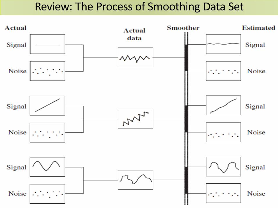
Review: The Process of Smoothing Data Set

Outline Konsep dasar pemulusan eksponensial

Pemulusan eksponensial sederhana

Peramalan melalui pemulusan eksponensialsederhana

Contoh aplikasi pada data

Moving Average Vs Exponential Smoothing

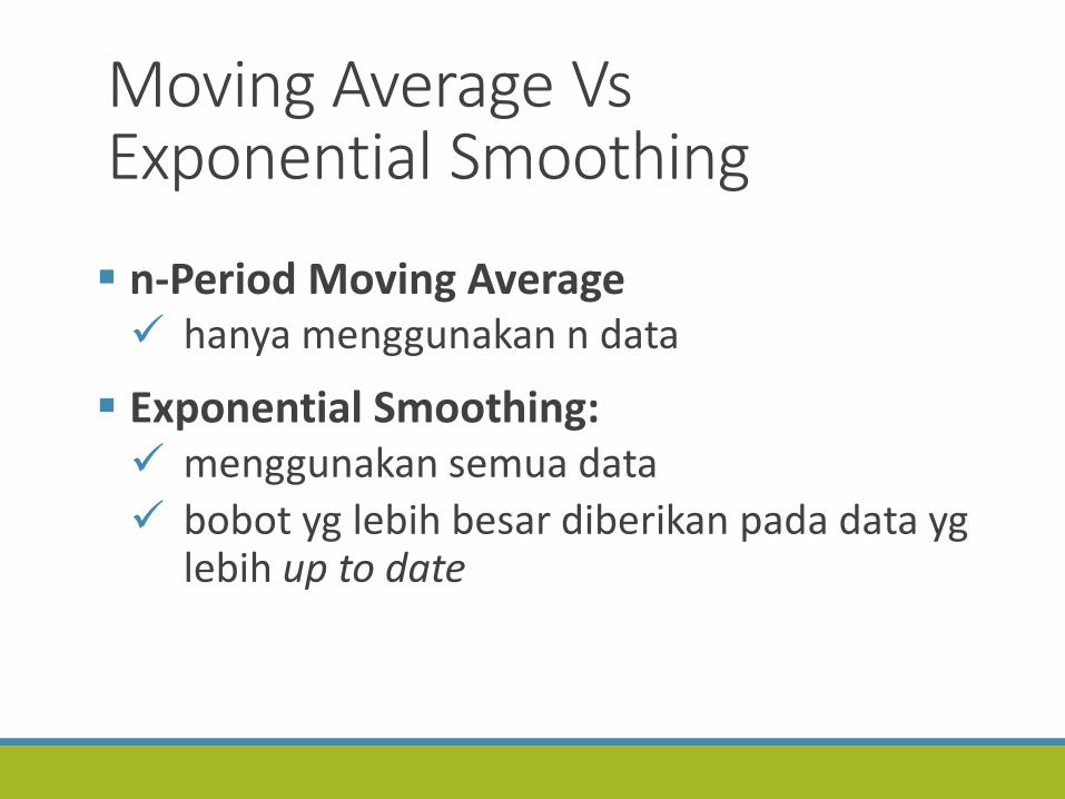
Moving Average Vs Exponential Smoothing

n‐Period Moving Average hanya menggunakan n data

Exponential Smoothing: menggunakan semua data

bobot yg lebih besar diberikan pada data yglebih up to date

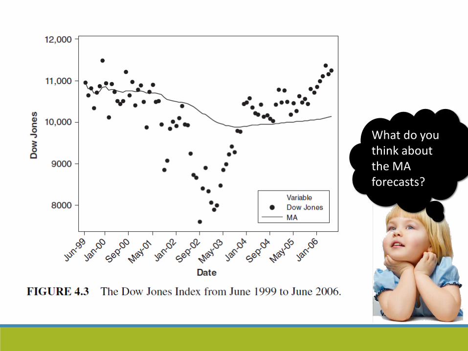
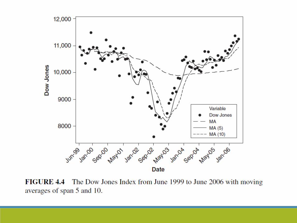
What do you think about the MA forecasts?

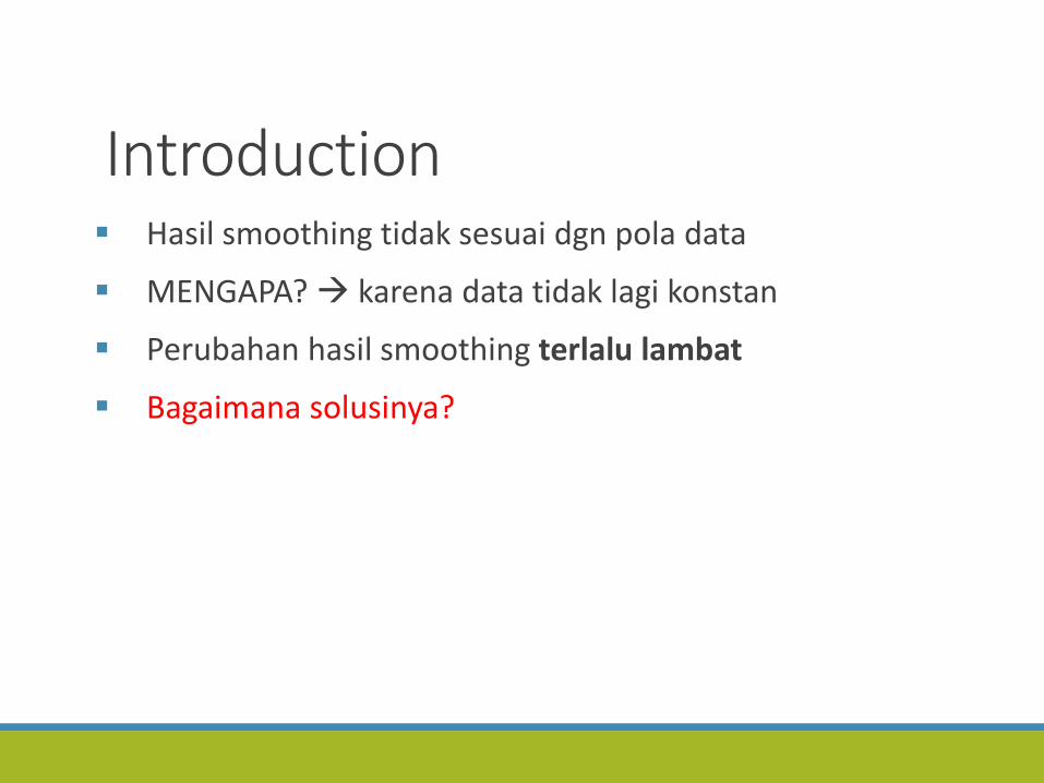
Introduction Hasil smoothing tidak sesuai dgn pola data

MENGAPA? karena data tidak lagi konstan

Perubahan hasil smoothing terlalu lambat

Bagaimana solusinya?

Konsep DasarPemulusan Eksponensial

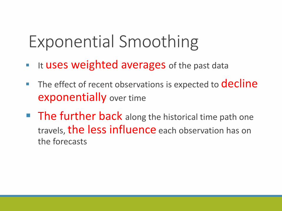
Exponential Smoothing It uses weighted averages of the past data

The effect of recent observations is expected to decline exponentially over time

The further back along the historical time path one

travels, the less influence each observation has on the forecasts

Pemulusan EksponensialSederhana(SINGLE EXPONENTIAL SMOOTHING)

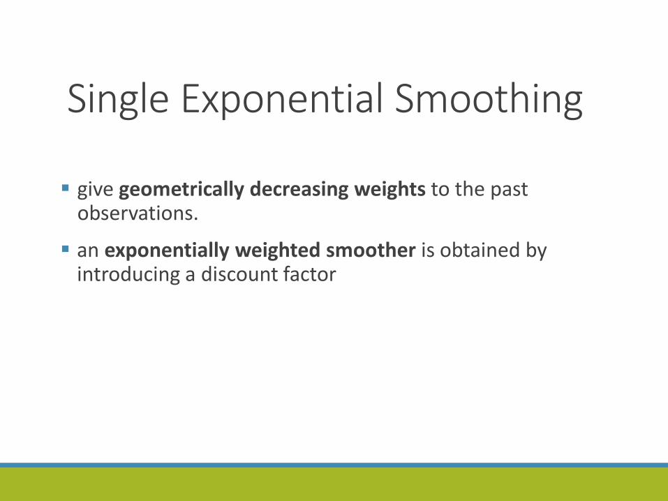
Single Exponential Smoothing

give geometrically decreasing weights to the past observations.

an exponentially weighted smoother is obtained by introducing a discount factor

Slide 14

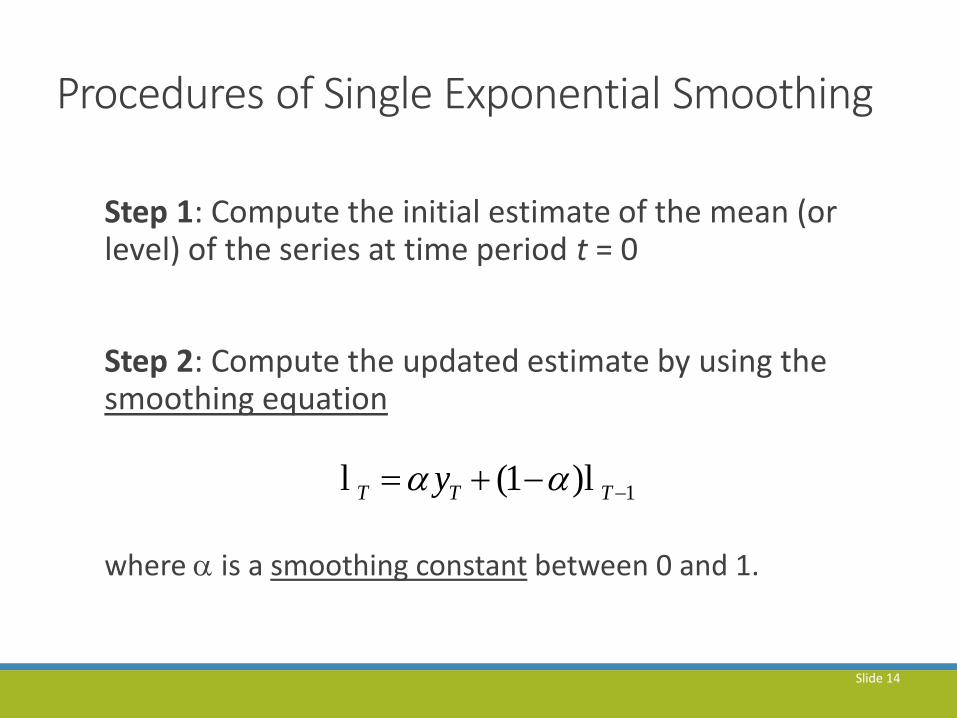
Procedures of Single Exponential Smoothing

Step 1: Compute the initial estimate of the mean (or level) of the series at time period t = 0

Step 2: Compute the updated estimate by using the smoothing equation

where is a smoothing constant between 0 and 1.

1(1 )T T Ty l l

Slide 15

Procedures of Single Exponential Smoothing

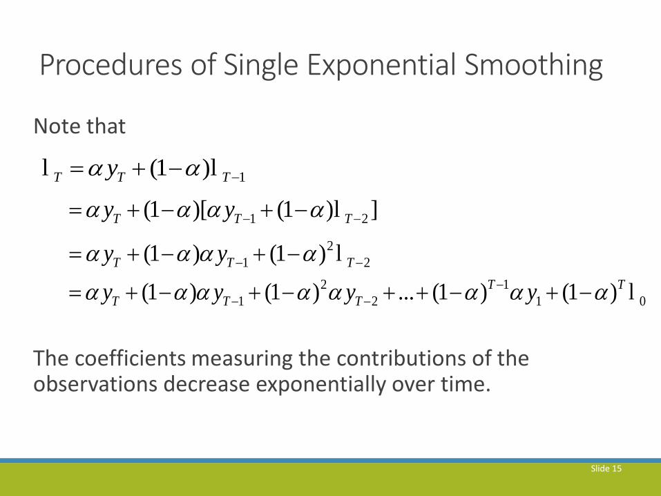
Note that

The coefficients measuring the contributions of the observations decrease exponentially over time.

1(1 )T T Ty l l

1 2(1 )[ (1 ) ]T T Ty y l

2

1 2(1 ) (1 )T T Ty y l

2 1

1 2 1 0(1 ) (1 ) ... (1 ) (1 )T T

T T Ty y y y

l

Single Exponential Smoothing

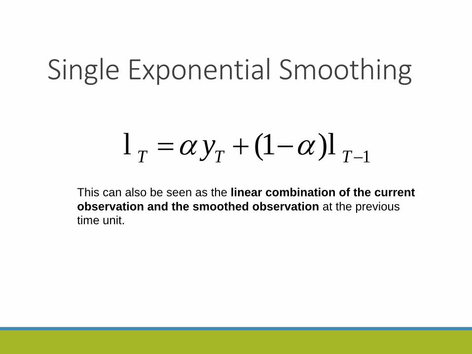
This can also be seen as the linear combination of the current

observation and the smoothed observation at the previous time unit.

1(1 )T T Ty l l

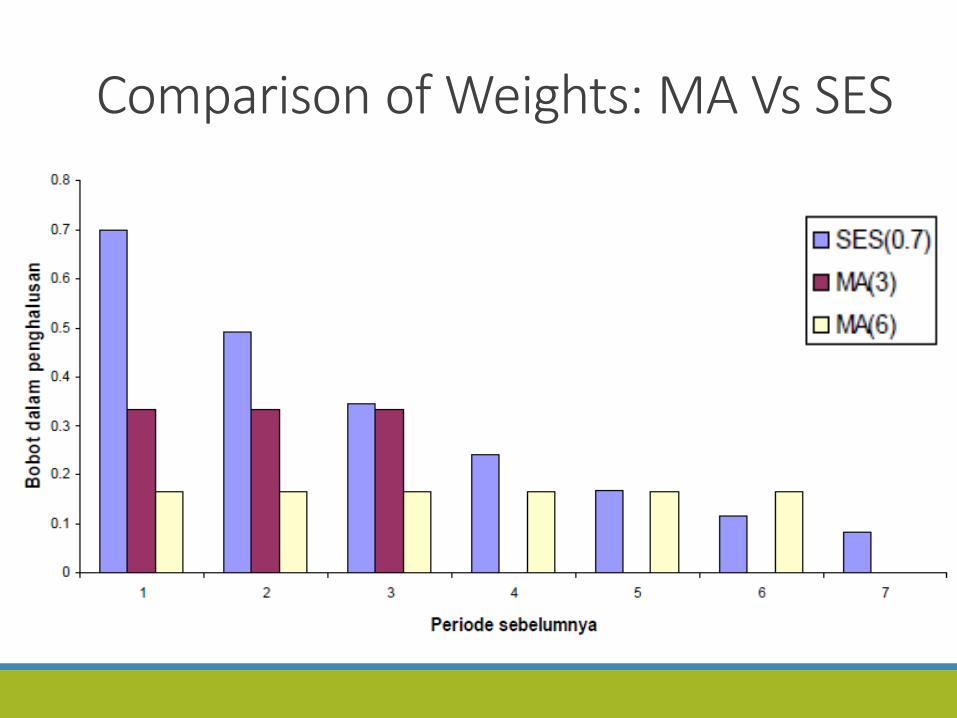
Comparison of Weights: MA Vs SES

Intial Value

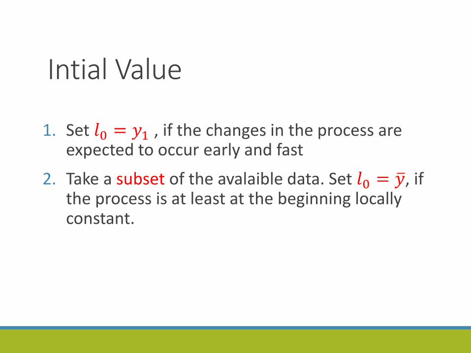
1. Set 𝑙0 = 𝑦1 , if the changes in the process are expected to occur early and fast

2. Take a subset of the avalaible data. Set 𝑙0 = 𝑦, if the process is at least at the beginning locally constant.

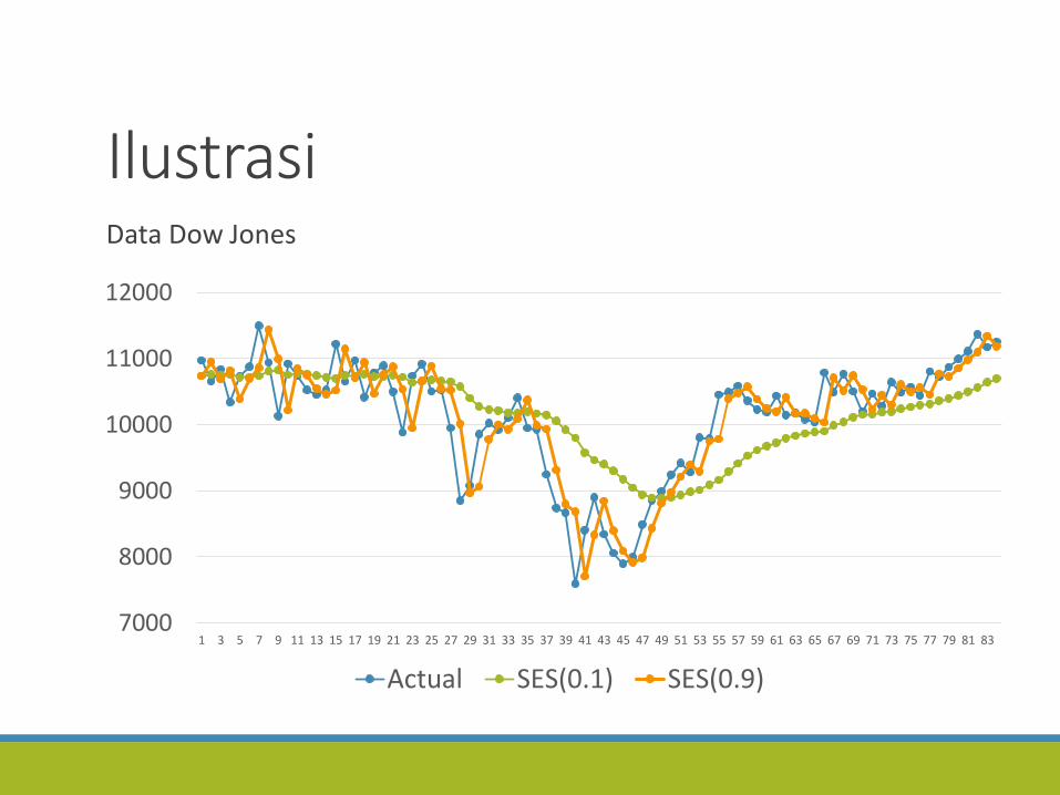
IlustrasiData Dow Jones

7000

8000

9000

10000

11000

12000

1 3 5 7 9 11 13 15 17 19 21 23 25 27 29 31 33 35 37 39 41 43 45 47 49 51 53 55 57 59 61 63 65 67 69 71 73 75 77 79 81 83

Actual SES(0.1) SES(0.9)

The Value of 𝛼 𝛼 → 0 maka hasil smoothing semakin smooth

𝛼 → 1 maka hasil smoothing semakin mendekatipola data aktual

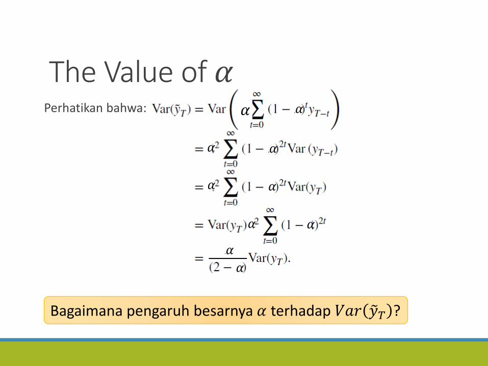
The Value of 𝛼Perhatikan bahwa:

Bagaimana pengaruh besarnya 𝛼 terhadap 𝑉𝑎𝑟 𝑦𝑇 ?

𝛼 𝛼

𝛼 𝛼

𝛼𝛼

𝛼 𝛼

𝛼

𝛼

The Value of 𝛼 Thus the question will be how much smoothing is

needed.

In the literature, 𝜶 values between 0.1 and 0.4 are often recommended and do indeed perform well in practice.

Peramalan

Slide 24

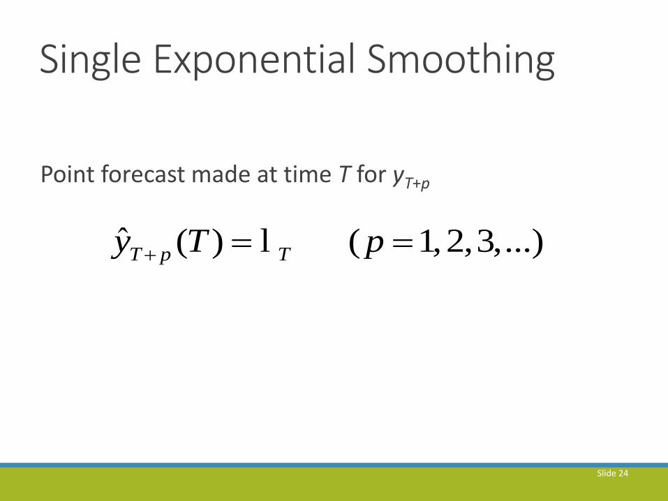
Single Exponential Smoothing

Point forecast made at time T for yT+p

ˆ ( ) ( 1,2,3,...)T p Ty T p l

Aplikasi pada Data

Slide 26

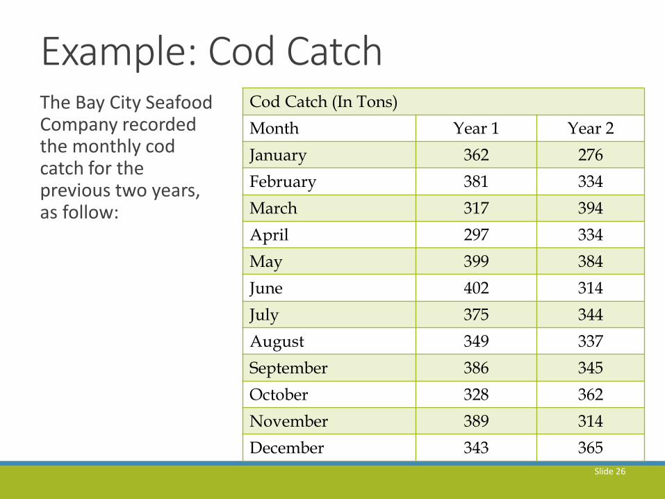
Example: Cod CatchThe Bay City Seafood Company recorded the monthly cod catch for the previous two years, as follow:

Cod Catch (In Tons)

Month Year 1 Year 2

January 362 276

February 381 334

March 317 394

April 297 334

May 399 384

June 402 314

July 375 344

August 349 337

September 386 345

October 328 362

November 389 314

December 343 365

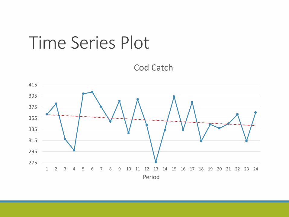
Time Series Plot

275

295

315

335

355

375

395

415

1 2 3 4 5 6 7 8 9 10 11 12 13 14 15 16 17 18 19 20 21 22 23 24

Period

Cod Catch

Time Series Plot

275

295

315

335

355

375

395

415

1 2 3 4 5 6 7 8 9 10 11 12 13 14 15 16 17 18 19 20 21 22 23 24

Period

Cod Catch

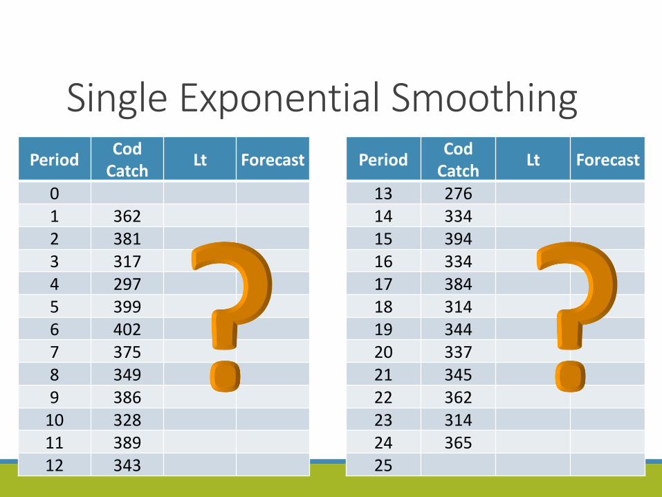
Single Exponential SmoothingPeriod

Cod Catch

Lt Forecast

01 3622 3813 3174 2975 3996 4027 3758 3499 386

10 32811 38912 343

PeriodCod

CatchLt Forecast

13 27614 33415 39416 33417 38418 31419 34420 33721 34522 36223 31424 36525

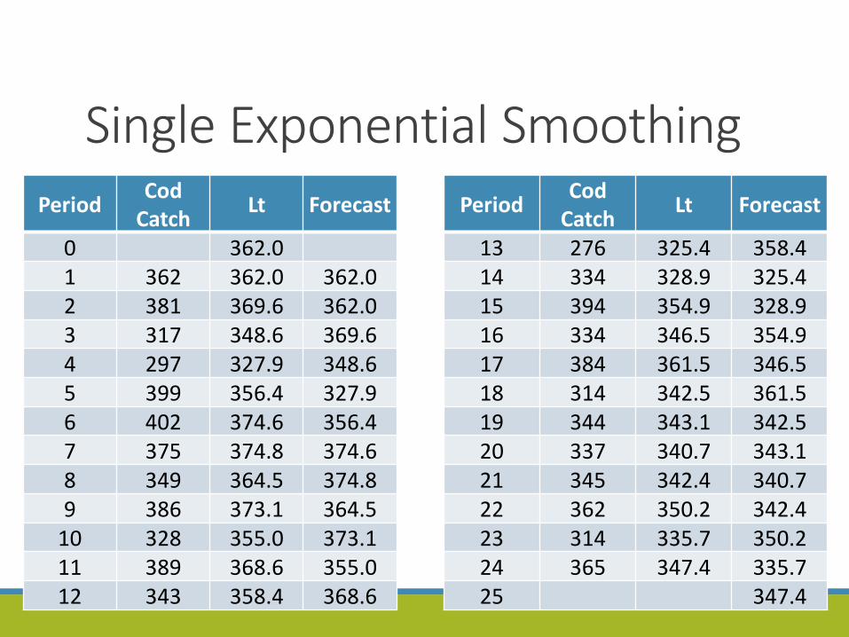
Single Exponential SmoothingPeriod

Cod Catch

Lt Forecast

0 362.01 362 362.0 362.02 381 369.6 362.03 317 348.6 369.64 297 327.9 348.65 399 356.4 327.96 402 374.6 356.47 375 374.8 374.68 349 364.5 374.89 386 373.1 364.5

10 328 355.0 373.111 389 368.6 355.012 343 358.4 368.6

PeriodCod

CatchLt Forecast

13 276 325.4 358.414 334 328.9 325.415 394 354.9 328.916 334 346.5 354.917 384 361.5 346.518 314 342.5 361.519 344 343.1 342.520 337 340.7 343.121 345 342.4 340.722 362 350.2 342.423 314 335.7 350.224 365 347.4 335.725 347.4

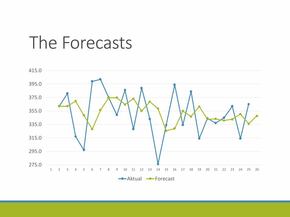
The Forecasts

275.0

295.0

315.0

335.0

355.0

375.0

395.0

415.0

1 2 3 4 5 6 7 8 9 10 11 12 13 14 15 16 17 18 19 20 21 22 23 24 25 26

Aktual Forecast

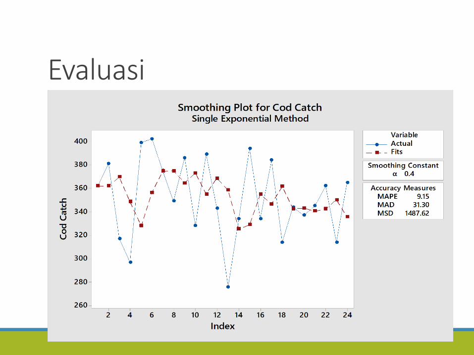
Evaluasi

Latihan1) Exercise 4.1 in Montgomery et al. (2015)

2) Exercise 4.2 in Montgomery et al. (2015)

ReferensiMontgomery, D.C., Jennings, C.L., Kulahci, M. 2015.

Introduction to Time Series Analysis andForecasting, 2nd ed. New Jersey: John Wiley &Sons.

34

Materi perkuliahan dapatdiakses pada:

stat.ipb.ac.id/en

35