lecture 12 - dualitytyu/math690optimization/lec12.pdf · lecture 12 - duality f = min f(x) s.t. g...

Lecture 12 - Duality

f ∗ = min f (x)s.t. gi (x) ≤ 0, i = 1, 2, . . . ,m

hj(x) = 0, j = 1, 2, . . . , p,x ∈ X ,

(1)

I f , gi , hj(i = 1, 2, . . . ,m, j = 1, 2, . . . , p) are functions defined on the setX ⊆ Rn.

I Problem (1) will be referred to as the primal problem.

I The Lagrangian is

L(x,λ,µ) = f (x) +m∑i=1

λigi (x) +

p∑j=1

µjhj(x) (x ∈ X ,λ ∈ Rm+,µ ∈ Rp)

I The dual objective function q : Rm+ × Rp → R ∪ {−∞} is defined to be

q(λ,µ) = minx∈X

L(x,λ,µ). (2)

Amir Beck “Introduction to Nonlinear Optimization” Lecture Slides - Duality 1 / 46

Thomas

Typewritten Text

Key observation: any such q(lambda, mu) is a LOWER BOUND for f* !

Thomas

Typewritten Text

Thomas

Typewritten Text

Thomas

Line

Thomas

Line

Thomas

Typewritten Text

(this minimum may not be attained)

Thomas

Typewritten Text

Thomas

Typewritten Text

Thomas

Typewritten Text

Thomas

Typewritten Text

The Dual Problem

I The domain of the dual objective function is

dom(q) = {(λ,µ) ∈ Rm+ × Rp : q(λ,µ) > −∞}.

I The dual problem is given by

q∗ = max q(λ,µ)s.t. (λ,µ) ∈ dom(q)

(3)


Convexity of the Dual Problem

Theorem. Consider problem (1) with f , gi , hj(i = 1, 2, . . . ,m, j =1, 2, . . . , p) being functions defined on the set X ⊆ Rn, and let q be thedual function defined in (2). Then

(a) dom(q) is a convex set.

(b) q is a concave function over dom(q).

Proof.

I (a) Take (λ1,µ1), (λ2,µ2) ∈ dom(q) and α ∈ [0, 1]. Then

minx∈X

L(x,λ1,µ1) > −∞, (4)

minx∈X

L(x,λ2,µ2) > −∞. (5)


Thomas

Typewritten Text

Thomas

Typewritten Text

Thomas

Typewritten Text

(even the primal problem is not convex)

Thomas

Typewritten Text

Thomas

Typewritten Text

Proof Contd.I Therefore, since the Lagrangian L(x,λ,µ) is affine w.r.t. λ,µ,

q(αλ1 + (1− α)λ2, αµ1 + (1− α)µ2)

= minx∈X

L(x, αλ1 + (1− α)λ2, αµ1 + (1− α)µ2)

= minx∈X{αL(x,λ1,µ1) + (1− α)L(x,λ2,µ2)}

≥ αminx∈X

L(x,λ,µ1) + (1− α) minx∈X

L(x,λ2,µ2)

= αq(λ1,µ1) + (1− α)q(λ2,µ2)

> −∞.

I Hence, α(λ1,µ1) + (1− α)(λ2,µ2) ∈ dom(q), and the convexity of dom(q)is established.

I (b) L(x,λ,µ) is an affine function w.r.t. (λ,µ).

I In particular, it is a concave function w.r.t. (λ,µ).

I Hence, since q is the minimum of concave functions, it must be concave.


Thomas

Typewritten Text

The Weak Duality TheoremTheorem. Consider the primal problem (1) and its dual problem (3). Then

q∗ ≤ f ∗,

where f ∗, q∗ are the primal and dual optimal values respectively.

Proof.I The feasible set of the primal problem is

S = {x ∈ X : gi (x) ≤ 0, hj(x) = 0, i = 1, 2, . . . ,m, j = 1, 2, . . . , p}.

I Then for any (λ,µ) ∈ dom(q) we have

q(λ,µ) = minx∈X

L(x,λ,µ) ≤ minx∈S

L(x,λ,µ)

= minx∈S

{f (x) +

m∑i=1

λigi (x) +

p∑j=1

µjhj(x)

}≤ min

x∈Sf (x) = f ∗.

I Taking the maximum over (λ,µ) ∈ dom(q), the result follows.Amir Beck “Introduction to Nonlinear Optimization” Lecture Slides - Duality 5 / 46

Thomas

Typewritten Text

Thomas

Typewritten Text

Thomas

Typewritten Text

Example

min x21 − 3x2

2

s.t. x1 = x32 .

In class


Thomas

Typewritten Text

It shows that q* can be an extremely poor lower bound for f*.

Strong Duality in the Convex Case - Back to SeparationSupporting Hyperplane Theorem Let C ⊆ Rn be a convex set and let y /∈ C .Then there exists 0 6= p ∈ Rn such that

pTx ≤ pTy for any x ∈ C .

Proof.I Although the theorem holds for any convex set C, we will prove it only for

sets with a nonempty interior.I Since y /∈ int(C ), it follows that y /∈ int(cl(C )).I Therefore, there exists a sequence {yk}k≥1 such that yk /∈ cl(C ) and yk → y.I By the separation theorem of a point from a closed and convex set, there

exists 0 6= pk ∈ Rn such that

pTk x < pTk yk ∀x ∈ cl(C )

I Thus,pTk‖pk‖

(x− yk) < 0 for any x ∈ cl(C ). (6)


Thomas

Typewritten Text

Thomas

Typewritten Text

As C is not required to be closed, y can be on the boundary of C.

Thomas

Typewritten Text

Proof Contd.

I Since the sequence{

pk‖pk‖

}is bounded, it follows that there exists a

subsequence{

pk‖pk‖

}k∈T

such that pk‖pk‖ → p as k

T−→∞ for some p ∈ Rn.

I Obviously, ‖p‖ = 1 and hence in particular p 6= 0.

I Taking the limit as kT−→∞ in inequality (6) we obtain that

pT (x− y) ≤ 0 for any x ∈ cl(C ),

which readily implies the result since C ⊆ cl(C ).


Thomas

Typewritten Text

Separation of Two Convex Sets

Theorem. Let C1,C2 ⊆ Rn be two nonempty convex sets such that C1∩C2 =∅. Then there exists 0 6= p ∈ Rn for which

pTx ≤ pTy for any x ∈ C1, y ∈ C2.

Proof.

I The set C1 − C2 is a convex set.

I C1 ∩ C2 = ∅ ⇒ 0 /∈ C1 − C2.

I By the supporting hyperplane theorem, there exists 0 6= p ∈ Rn such that

pT (x− y) ≤ pT0 for any x ∈ C1, y ∈ C2,


Thomas

Typewritten Text

The Nonlinear Farkas Lemma

Theorem. Let X ⊆ Rn be a convex set and let f , g1, g2, . . . , gm be convexfunctions over X . Assume that there exists x ∈ X such that

g1(x) < 0, g2(x) < 0, . . . , gm(x) < 0.

Let c ∈ R. Then the following two claims are equivalent:

(a) the following implication holds:

x ∈ X , gi (x) ≤ 0, i = 1, 2, . . . ,m⇒ f (x) ≥ c .

(b) there exist λ1, λ2, . . . , λm ≥ 0 such that

minx∈X

{f (x) +

m∑i=1

λigi (x)

}≥ c . (7)


Thomas

Typewritten Text

Thomas

Typewritten Text

Proof of (b)⇒ (a)

I Suppose that there exist λ1, λ2, . . . , λm ≥ 0 such that (7) holds, and letx ∈ X satisfy gi (x) ≤ 0, i = 1, 2, . . . ,m.

I By (7) we have

f (x) +m∑i=1

λigi (x) ≥ c ,

I Hence,

f (x) ≥ c −m∑i=1

λigi (x) ≥ c .


Thomas

Typewritten Text

(The is the easier step, which does not require convexity.)

Thomas

Typewritten Text

Thomas

Typewritten Text

Thomas

Typewritten Text

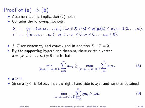
Proof of (a) ⇒ (b)I Assume that the implication (a) holds.I Consider the following two sets:

S = {u = (u0, u1, . . . , um) : ∃x ∈ X , f (x) ≤ u0, gi (x) ≤ ui , i = 1, 2, . . . ,m},T = {(u0, u1, . . . , um) : u0 < c , u1 ≤ 0, u2 ≤ 0, . . . , um ≤ 0}.

I S ,T are nonempty and convex and in addition S ∩ T = ∅.I By the supporting hyperplane theorem, there exists a vector

a = (a0, a1, . . . , am) 6= 0, such that

min(u0,u1,...,um)∈S

m∑j=0

ajuj ≥ max(u0,u1,...,um)∈T

m∑j=0

ajuj . (8)

I a ≥ 0.I Since a ≥ 0, it follows that the right-hand side is a0c , and we thus obtained


m∑j=0

ajuj ≥ a0c . (9)


Thomas

Typewritten Text

Thomas

Typewritten Text

Thomas

Typewritten Text

Thomas

Typewritten Text

Proof of (a) ⇒ (b) Contd.I We will show that a0 > 0. Suppose in contradiction that a0 = 0. Then

min(u0,u1,...,um)∈S∑m

j=1 ajuj ≥ 0.I Since we can take ui = gi (x), we can deduce that

∑mj=1 ajgj(x) ≥ 0, which is

impossible since gj(x) < 0 and a 6= 0.I Since a0 > 0, we can divide (9) by a0 to obtain


u0 +m∑j=1

ajuj

≥ c , (10)

where aj =aja0

.I By the definition of S we have


u0 +m∑j=1

ajuj

≤ minx∈X

f (x) +m∑j=1

ajgj(x)

,

which combined with (10) yields the desired result

minx∈X

f (x) +m∑j=1

ajgj(x)

≥ c .


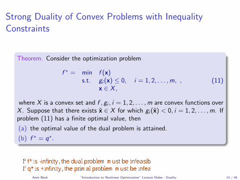
Strong Duality of Convex Problems with InequalityConstraints

Theorem. Consider the optimization problem

f ∗ = min f (x)s.t. gi (x) ≤ 0, i = 1, 2, . . . ,m,

x ∈ X ,, (11)

where X is a convex set and f , gi , i = 1, 2, . . . ,m are convex functions overX . Suppose that there exists x ∈ X for which gi (x) < 0, i = 1, 2, . . . ,m. Ifproblem (11) has a finite optimal value, then

(a) the optimal value of the dual problem is attained.

(b) f ∗ = q∗.


Thomas

Typewritten Text

Easy consequences of weak duality: If f* is -infinity, the dual problem must be infeasible. If q* is +infinity, the primal problem must be infeasible.

Thomas

Typewritten Text

Thomas

Typewritten Text

Thomas

Line

Thomas

Line

Proof of Strong Duality TheoremI Since f ∗ > −∞ is the optimal value of (11), it follows that the following

implication holds:

x ∈ X , gi (x) ≤ 0, i = 1, 2, . . . ,m⇒ f (x) ≥ f ∗,

I By the nonlinear Farkas Lemma there exists λ1, λ2, . . . , λm ≥ 0 such that

q(λ) = minx∈X

f (x) +m∑j=1

λjgj(x)

≥ f ∗.

I By the weak duality theorem,

q∗ ≥ q(λ) ≥ f ∗ ≥ q∗,

I Hence f ∗ = q∗ and λ is an optimal solution of the dual problem.


Thomas

Typewritten Text

Example

min x21 − x2

s.t. x22 ≤ 0.

In class


Thomas

Callout

fails Slater condition

Thomas

Typewritten Text

Will show: f* = q*, but the dual problem does not have a maximizer.

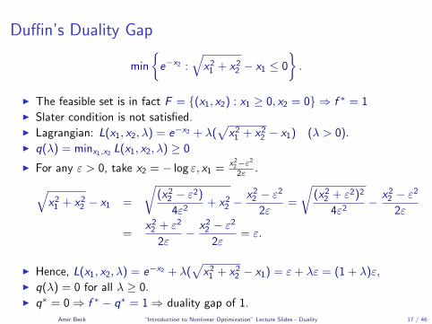
Duffin’s Duality Gap

min

{e−x2 :

√x2

1 + x22 − x1 ≤ 0

}.

I The feasible set is in fact F = {(x1, x2) : x1 ≥ 0, x2 = 0} ⇒ f ∗ = 1I Slater condition is not satisfied.I Lagrangian: L(x1, x2, λ) = e−x2 + λ(

√x2

1 + x22 − x1) (λ > 0).

I q(λ) = minx1,x2 L(x1, x2, λ) ≥ 0

I For any ε > 0, take x2 = − log ε, x1 =x2

2−ε2

2ε .√x2

1 + x22 − x1 =

√(x2

2 − ε2)

4ε2+ x2

2 −x2

2 − ε2

2ε=

√(x2

2 + ε2)2

4ε2− x2

2 − ε2

2ε

=x2

2 + ε2

2ε− x2

2 − ε2

2ε= ε.

I Hence, L(x1, x2, λ) = e−x2 + λ(√x2

1 + x22 − x1) = ε+ λε = (1 + λ)ε,

I q(λ) = 0 for all λ ≥ 0.I q∗ = 0⇒ f ∗ − q∗ = 1⇒ duality gap of 1.


Thomas

Callout

also implies it is a convex problem

Thomas

Callout

>=0

Thomas

Typewritten Text

(i.e. x1 >> x2 -> infinity)

Thomas

Typewritten Text

(If we make x2 arbitrarily big (then exp(-x2) gets arbitrarily small). If, furthermore, we make x1 way bigger than x2, then the second term also gets arbitrarily small also.)

Thomas

Typewritten Text

(we shall see the inf. is 0 for any lambda, but a minimizer doesn't exist.)

Thomas

Typewritten Text

Thomas

Typewritten Text

Thomas

Typewritten Text

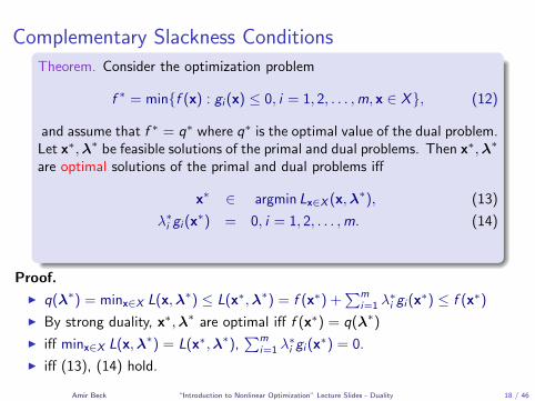
Complementary Slackness Conditions

Theorem. Consider the optimization problem

f ∗ = min{f (x) : gi (x) ≤ 0, i = 1, 2, . . . ,m, x ∈ X}, (12)

and assume that f ∗ = q∗ where q∗ is the optimal value of the dual problem.Let x∗,λ∗ be feasible solutions of the primal and dual problems. Then x∗,λ∗

are optimal solutions of the primal and dual problems iff

x∗ ∈ argmin Lx∈X (x,λ∗), (13)

λ∗i gi (x∗) = 0, i = 1, 2, . . . ,m. (14)

Proof.

I q(λ∗) = minx∈X L(x,λ∗) ≤ L(x∗,λ∗) = f (x∗) +∑m

i=1 λ∗i gi (x

∗) ≤ f (x∗)

I By strong duality, x∗,λ∗ are optimal iff f (x∗) = q(λ∗)

I iff minx∈X L(x,λ∗) = L(x∗,λ∗),∑m

i=1 λ∗i gi (x

∗) = 0.

I iff (13), (14) hold.


Thomas

Typewritten Text

A More General Strong Duality TheoremTheorem. Consider the optimization problem

f ∗ = min f (x)s.t. gi (x) ≤ 0, i = 1, 2, . . . ,m,

hj(x) ≤ 0, j = 1, 2, . . . , p,sk(x) = 0, k = 1, 2, . . . , q,x ∈ X ,

(15)

where X is a convex set and f , gi , i = 1, 2, . . . ,m are convex functionsover X . The functions hj , sk are affine functions. Suppose that there existsx ∈ int(X ) for which gi (x) < 0, hj(x) ≤ 0, sk(x) = 0. Then if problem (15)has a finite optimal value, then the optimal value of the dual problem

q∗ = max{q(λ,η,µ) : (λ,η,µ) ∈ dom(q)},

where

q(λ,η,µ) = minx∈X

[f (x) +

∑mi=1 λigi (x) +

∑pj=1 ηjhj(x) +

∑qk=1 µksk(x)

]is attained, and f ∗ = q∗.


Thomas

Typewritten Text

Importance of the Underlying Set

(P)min x3

1 + x32

s.t. x1 + x2 ≥ 1,x1, x2 ≥ 0.

I ( 12 ,

12 ) is the optimal solution of (P) with an optimal value f ∗ = 1

4 .

I First dual problem is constructed by taking X = {(x1, x2) : x1, x2 ≥ 0}.I The primal problem is min{x3

1 + x32 : x1 + x2 ≥ 1, (x1, x2) ∈ X}.

I Strong duality holds for the problem and hence in particular q∗ = 14 .

I Second dual is constructed by taking X = R2.

I Objective function is not convex ⇒ strong duality is not necessarily satisfied.

I L(x1, x2, λ, η1, η2) = x31 + x3

2 − λ(x1 + x2 − 1)− η1x1 − η2x2.

I q(λ, η1, η2) = −∞ for all (λ, µ1, µ2) ⇒ q∗ = −∞.


Thomas

Line

Thomas

Line

Thomas

Callout

f is not convex on it

Thomas

Callout

f(x1,x2)

Thomas

Callout

f is convex on this X

Linear ProgrammingConsider the linear programming problem

min cTxs.t. Ax ≤ b,

I c ∈ Rn,A ∈ Rm×n and b ∈ Rm.

I We assume that the problem is feasible ⇒ strong duality holds.

I L(x,λ) = cTx + λT (Ax− b) = (c + ATλ)Tx− bTλ.

I Dual objective funvtion:

q(λ) = minx∈Rn

L(x,λ) = minx∈Rn

(c+ATλ)Tx−bTλ =

{−bTλ c + ATλ = 0,−∞ else.

I Dual problem:max −bTλs.t. ATλ = −c,

λ ≥ 0.


Thomas

Typewritten Text

Thomas

Typewritten Text

Thomas

Typewritten Text

Strictly Convex Quadratic ProgrammingConsider the strictly convex quadratic programming problem

min xTQx + 2fTxs.t. Ax ≤ b,

(16)

I Q ∈ Rn×n positive definite, f ∈ Rn,A ∈ Rm×n, b ∈ Rm.I Lagrangian: (λ ∈ Rm

+) L(x,λ) = xTQx + 2fTx + 2λT (Ax− b) =xTQx + 2(ATλ + f)Tx− 2bTλ.

I The minimizer of the Lagrangian is attained at x∗ = −Q−1(f + ATλ).I

q(λ) = L(x∗,λ)

= (f + ATλ)TQ−1QQ−1(f + ATλ)− 2(f + ATλ)TQ−1(f + ATλ)− 2bTλ

= −(f + ATλ)TQ−1(f + ATλ)− 2bTλ

= −λTAQ−1ATλ− 2fTQ−1ATλ− fTQ−1f − 2bTλ

= −λTAQ−1ATλ− 2(AQ−1f + b)Tλ− fTQ−1f.

I The dual problem is max{q(λ) : λ ≥ 0}.Amir Beck “Introduction to Nonlinear Optimization” Lecture Slides - Duality 22 / 46

Dual of Convex QCQP with strictly convex objectiveConsider the QCQP problem

min xTA0x + 2bT0 x + c0

s.t. xTAix + 2bTi x + ci ≤ 0, i = 1, 2, . . . ,m,

where Ai � 0 is an n × n matrix, bi ∈ Rn, ci ∈ R, i = 0, 1, . . . ,m.Assume that A0 � 0.

I Lagrangian (λ ∈ Rm+):

L(x,λ) = xTA0x+ 2bT0 x+ c0 +

m∑i=1

λi (xTAix+ 2bT

i x+ ci )

= xT(A0 +

∑mi=1 λiAi

)x+ 2

(b0 +

∑mi=1 λibi

)Tx+ c0 +

∑mi=1 λici .

I The minimizer of the Lagrangian w.r.t. x is attained at x satisfying

2(A0 +

∑mi=1 λiAi

)x = −2

(b0 +

∑mi=1 λibi

).

I Thus, x = −(A0 +

∑mi=1 λiAi

)−1 (b0 +

∑mi=1 λibi

).


QCQP contd.

I Plugging this expression back into the Lagrangian, we obtain the followingexpression for the dual objective function

q(λ) = minx

L(x,λ) = L(x,λ)

= xT(A0 +

∑mi=1 λiAi

)x+ 2

(b0 +

∑mi=1 λibi

)Tx+ c0 +

∑mi=1 λici

= −(b0 +

∑mi=1 λibi

)T (A0 +

∑mi=1 λiAi

)−1 (b0 +

∑mi=1 λibi

)+

c0 +∑m

i=1 λici .

I The dual problem is thus

max −(b0 +

∑mi=1 λibi

)T (A0 +

∑mi=1 λiAi

)−1 (b0 +

∑mi=1 λibi

)+

c0 +∑m

i=1 λicis.t. λi ≥ 0, i = 1, 2, . . . ,m.


Dual of Convex QCQPs

A0 is only assumed to be positive semidefinite.

I The previous dual is not well defined since the matrix A0 +∑m

i=1 λiAi is notnecessarily PD.

I Decompose Ai as Ai = DTi Di (Di ∈ Rn×n) and rewrite the problem as

min xTDT0 D0x + 2bT0 x + c0

s.t. xTDTi Dix + 2bTi x + ci ≤ 0, i = 1, 2, . . . ,m,

I Define additional variables zi = Dix, giving rise to the formulation

min ‖z0‖2 + 2bT0 x + c0

s.t. ‖zi‖2 + 2bTi x + ci ≤ 0, i = 1, 2, . . . ,m,zi = Dix, i = 0, 1, . . . ,m.


Dual of Convex QCQPsI The Lagrangian is (λ ∈ Rm

+,µi ∈ Rn, i = 0, 1, . . . ,m):

L(x, z0, . . . , zm,λ,µ0, . . . ,µm)

= ‖z0‖2 + 2bT0 x + c0 +m∑i=1

λi (‖zi‖2 + 2bTi x + ci ) +

2m∑i=0

µTi (zi −Dix)

= ‖z0‖2 + 2µT0 z0 +

m∑i=1

(λi‖zi‖2 + 2µTi zi ) +

2

(b0 +

m∑i=1

λibi −m∑i=0

DTi µi

)T

x

+c0 +m∑i=1

ciλi .


Dual of Convex QCQPsI For any λ ∈ R+,µ ∈ Rn,

g(λ,µ) ≡ minz

{λ‖z‖2 + 2µT z

}=

−‖µ‖2

λ λ > 0,0 λ = 0,µ = 0,−∞ λ = 0,µ 6= 0.

I Since the Lagrangian is separable with respect to zi and x, we can performthe minimization with respect to each of the variables vectors:

minz0

[‖z0‖2 + 2µT

0 z0

]= g(1,µ0) = −‖µ0‖2,

minzi

[λi‖zi‖2 + 2µT

i zi]

= g(λi ,µi ),

minx

(b0 +

∑mi=1 λibi −

∑mi=0 D

Ti µi

)Tx =

{0 b0 +

∑mi=1 λibi −

∑mi=0 D

Ti µi = 0,

−∞ else,

I Hence,

q(λ,µ0, . . . ,µm) = minx,z0,...,zm

L(x, z0, . . . , zm,λ,µ0, . . . ,µm)

=

{g(1,µ0) +

∑mi=1 g(λi ,µi ) + c0 + cTλ b0 +

∑mi=1 λibi −

∑mi=0 D

Ti µi = 0,

−∞ else.


Dual of Convex QCQPs

The dual problem is therefore

max g(1,µ0) +∑m

i=1 g(λi ,µi ) + c0 +∑m

i=1 ciλis.t. b0 +

∑mi=1 λibi −

∑mi=0 D

Ti µi = 0,

λ ∈ Rm+,µ0, . . . ,µm ∈ Rn.


Dual of Nonconvex QCQPsConsider the problem

min xTA0x + 2bT0 x + c0

s.t. xTAix + 2bTi x + ci ≤ 0, i = 1, 2, . . . ,m,

I Ai = ATi ∈ Rn×n,bi ∈ Rn, ci ∈ R, i = 0, 1, . . . ,m.

I We do not assume that Ai are positive semidefinite, and hence the problem isin general nonconvex.

I Lagrangian (λ ∈ Rm+):

L(x,λ) = xTA0x+ 2bT0 x+ c0 +

m∑i=1

λi

(xTAix+ 2bT

i x+ ci)

= xT(A0 +

m∑i=1

λiAi

)x+ 2

(b0 +

m∑i=1

λibi

)T

x+ c0 +m∑i=1

ciλi .

I Note that

q(λ) = minx

L(x,λ) = maxt{t : L(x,λ) ≥ t for any x ∈ Rn}.


Dual of Nonconvex QCQPs

I The following holds:L(x,λ) ≥ t for all x ∈ Rn

is equivalent to(A0 +

∑mi=1 λiAi b0 +

∑mi=1 λibi

(b0 +∑m

i=1 λibi )T c0 +

∑mi=1 λici − t

)� 0,

I Therefore, the dual problem is

maxt,λi t

s.t.

(A0 +

∑mi=1 λiAi b0 +

∑mi=1 λibi

(b0 +∑m

i=1 λibi )T c0 +

∑mi=1 λici − t

)� 0,

λi ≥ 0, i = 1, 2, . . . ,m.


Orthogonal Projection onto the Unit SimplexI Given a vector y ∈ Rn, the orthogonal projection of y onto ∆n is the solution

tomin ‖x− y‖2

s.t. eTx = 1,x ≥ 0.

I Lagrangian:

L(x, λ) = ‖x− y‖2 + 2λ(eTx− 1) = ‖x‖2 − 2(y − λe)Tx + ‖y‖2 − 2λ

=n∑

j=1

(x2j − 2(yj − λ)xj) + ‖y‖2 − 2λ.

I The optimal xj is the solution to the 1D problem minxj≥0[x2j − 2(yj − λ)xj ].

I The optimal xj is xj =

{yj − λ yj ≥ λ0 else

= [yj − λ]+, with optimal value

−[yj − λ]2+.

I The dual problem is

maxλ∈R

{g(λ) ≡ −

∑nj=1[yj − λ]2

+ − 2λ+ ‖y‖2}.


Orthogonal Projection onto the Unit Simplex

I g is concave, differentiable, limλ→∞ g(λ) = limλ→−∞ g(λ) = −∞.I Therefore, there exists an optimal solution to the dual problem attained at a

point λ∗ in which g ′(λ∗) = 0.

I∑n

j=1[yj − λ∗]+ = 1.

I h(λ) =∑n

j=1[yj − λ]+ − 1 is nonincreasing over R and is in fact strictlydecreasing over (−∞,maxj yj ].

I

h (ymax) = −1,

h

(ymin −

2

n

)=

n∑j=1

yj − nymin + 2− 1 > 0,

where ymax = maxj=1,2,...,n yj , ymin = minj=1,2,...,n yj .

I We can therefore invoke a bisection procedure to find the unique root λ∗ ofthe function h over the interval [ymin − 2

n , ymax], and then defineP∆n(y) = [y − λ∗e]+.


Orthogonal Projection Onto the Unit Simplex

The MATLAB function proj_unit_simplex:

function xp=proj_unit_simplex(y)

f=@(lam)sum(max(y-lam,0))-1;

n=length(y);

lb=min(y)-2/n;

ub=max(y);

lam=bisection(f,lb,ub,1e-10);

xp=max(y-lam,0);


Dual of the Chebyshev Center ProblemI Formulation:

minx,r rs.t. ‖x− ai‖ ≤ r , i = 1, 2, . . . ,m.

I Reformulation:

minx,γ γs.t. ‖x− ai‖2 ≤ γ, i = 1, 2, . . . ,m.

I

L(x, γ,λ) = γ +m∑i=1

λi (‖x− ai‖2 − γ)

= γ(1−

∑mi=1 λi

)+∑m

i=1 λi‖x− ai‖2.

I The minimization of the above expression must be −∞ unless∑m

i=1 λi = 1,and in this case we have

minγγ

(1−

m∑i=1

λi

)= 0.


Dual of Chebyshev Center Contd.I Need to solve minx

∑mi=1 λi‖x− ai‖2.

I We have∑mi=1 λi‖x− ai‖2 = ‖x‖2 − 2

(∑mi=1 λiai

)Tx +

∑mi=1 λi‖ai‖2, (17)

I The minimum is attained at the point in which the gradient vanishes:

x∗ =m∑i=1

λiai = Aλ,

A is the n ×m matrix whose columns are a1, a2, . . . , am.I Substituting this expression back into (17),

q(λ) = ‖Aλ‖2 − 2(Aλ)T (Aλ) +∑m

i=1 λi‖ai‖2 = −‖Aλ‖2 +∑m

i=1 λi‖ai‖2.

I The dual problem is therefore

max −‖Aλ‖2 +∑m

i=1 λi‖ai‖2

s.t. λ ∈ ∆m.


MATLAB codefunction [xp,r]=chebyshev_center(A)

d=size(A);

m=d(2);

Q=A’*A;

L=2*max(eig(Q));

b=sum(A.^2)’;

%initialization with the uniform vector

lam=1/m*ones(m,1);

old_lam=zeros(m,1);

while (norm(lam-old_lam)>1e-5)

old_lam=lam;

lam=proj_unit_simplex(lam+1/L*(-2*Q*lam+b));

end

xp=A*lam;

r=0;

for i=1:m

r=max(r,norm(xp-A(:,i)));

endAmir Beck “Introduction to Nonlinear Optimization” Lecture Slides - Duality 36 / 46

Denoising

Suppose that we are given a signal contaminated with noise.

y = x + w,

x - unknown “true” signal, w - unknown noise, y - known observed signal.

The denoising problem: find a “good” estimate for x given y.


A Tikhonov Regularization Approach

Quadratic Penalty:

min ‖x− y‖2 + λ

n−1∑i=1

(xi − xi+1)2,

The solution with λ = 1:

Pretty good!


Weakness of Quadratic Regularization

The quadratic regularization method does not work so well for all types of signals.True and noisy step functions:


Failure of Quadratic Regularization


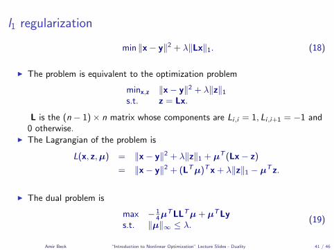
l1 regularization

min ‖x− y‖2 + λ‖Lx‖1. (18)

I The problem is equivalent to the optimization problem

minx,z ‖x− y‖2 + λ‖z‖1

s.t. z = Lx.

L is the (n − 1)× n matrix whose components are Li,i = 1, Li,i+1 = −1 and0 otherwise.

I The Lagrangian of the problem is

L(x, z,µ) = ‖x− y‖2 + λ‖z‖1 + µT (Lx− z)

= ‖x− y‖2 + (LTµ)Tx + λ‖z‖1 − µT z.

I The dual problem is

max − 14µ

TLLTµ + µTLys.t. ‖µ‖∞ ≤ λ.

(19)


A MATLAB code

Employing the gradient projection method on the dual:

lambda=1;

mu=zeros(n-1,1);

for i=1:1000

mu=mu-0.25*L*(L’*mu)+0.5*(L*y);

mu=lambda*mu./max(abs(mu),lambda);

xde=y-0.5*L’*mu;

end

figure(5)

plot(t,xde,’.’);

axis([0,1,-1,4])


l1-regularized solution


Dual of the Linear Separation Problem (Dual SVM)I x1, x2, . . . , xm ∈ Rn.

I For each i , we are given a scalar yi which is equal to 1 if xi is in class A or−1 if it is in class B.

I The problem of finding a maximal margin hyperplane that separates the twosets of points is

min 12‖w‖

2

s.t. yi (wTxi + β) ≥ 1, i = 1, 2, . . . ,m.

I The above assumes that the two classes are linearly seperable.

I A formulation that allows violation of the constraints (with an appropriatepenality):

min 12‖w‖

2 + C∑m

i=1 ξis.t. yi (wTxi + β) ≥ 1− ξi , i = 1, 2, . . . ,m,

ξi ≥ 0, i = 1, 2, . . . ,m,

where C > 0 is a penalty parameter.


Dual SVM

I The same asmin 1

2‖w‖2 + C (eTξ)

s.t. Y(Xw + βe) ≥ e− ξ,ξ ≥ 0,

where Y = diag(y1, y2, . . . , ym) and X is the m × n matrix whose rows arexT1 , x

T2 , . . . , x

Tm.

I Lagrangian (α ∈ Rm+):

L(w, β, ξ,α) =1

2‖w‖2 + C(eTξ)−αT [YXw + βYe− e+ ξ]

=1

2‖w‖2 − wT [XTYα]− β(αTYe) + ξT (Ce−α) +αTe.

I

q(α) =

[minw

1

2‖w‖2 − wT [XTYα]

]+

[minβ

(−β(αTYe))

]+

[minξ≥0

ξT (Ce−α)

]+αTe.


Dual SVMI

minw

1

2‖w‖2 −wT [XTYα] = −1

2αTYXXTYα,

minβ

(−β(αTYe)) =

{0 αTYe = 0,−∞ else,

minξ≥0

ξT (Ce−α) =

{0 α ≤ Ce,−∞ else,

I Therefore, the dual objective function is given by

q(α) =

{αTe− 1

2αTYXXTYα αTYe = 0, 0 ≤ α ≤ Ce

−∞ else.

I The dual problem ismax αTe− 1

2αTYXXTYα

s.t. αTYe = 0,0 ≤ α ≤ Ce.

I ormax

∑mi=1 αi − 1

2

∑mi=1

∑mj=1 αiαjyiyj(x

Ti xj)

s.t.∑m

i=1 yiαi = 0,0 ≤ αi ≤ C , i = 1, 2, . . . ,m.


lecture 12 - dualitytyu/math690optimization/lec12.pdf · lecture 12 - duality f = min f(x) s.t. g...

Documents