WORKING PAPER WP/11/2007

BUSINESS SURVEY AND POLICY INDICATORS

Donni Fajar Anugrah Ari Nopianti

November 2007

ii

iii

BUSINESS SURVEY AND POLICY INDICATORS

Donni Fajar Anugrah1, Ari Nopianti2

Working Paper Nomor 11

November 2007

ABSTRAKS

Paper ini bertujuan untuk memperoleh policy indicator yang terbaik dengan

menggunakan hasil dari business survey atau survey kegiatan dunia usaha (SKDU). Oleh

karena itu, perlu dilakukan perbaikan pada methode pengolahan data hasil survey

tersebut. Selain itu, dicoba juga untuk melakukan penyempurnaan bentuk survey tersebut

dengan mengkaji pertanyaan yang diajukan dalam kuesioner dan juga jumlah perusahaan

yang menjadi sample selama ini. Metode untuk memperoleh indikator tersebut

menggunakan principal component analysis (PCA), dimana diharapkan dapat

menggabungkan komposit dari jenis pertanyaan yang ada dalam kuesioner SKDU

tersebut.

JEL classification: E01, F32, C42,

Keywords: business survey, policy indicators, dan principal component anlysis

1 Peneliti Ekonomi di Biro Riset Ekonomi (BRE), Direktorat Riset Ekonomi dan Kebijakan Moneter (DKM), Bank Indonesia 2 Peneliti Ekonomi di Tim Statistik Sektor Riil (SSR), Direktorat Statistik Ekonomi dan Moneter (DSM), Bank Indonesia. Pandangan dalam paper ini merupakan pandangan penulis dan tidak merefleksikan pandangan DKM atau DSM atau Bank Indonesia. Kesalahan atau kekeliruan yang ada adalah kesalahan penulis: donni@bi.go.id dan arin@bi.go.id

iv

v

DAFTAR ISI

ABSTRAKS........................................................................................................................... iii DAFTAR ISI ........................................................................................................................... v DAFTAR GAMBAR............................................................................................................... vi DAFTAR TABEL.................................................................................................................... vi I. Introduction ................................................................................................................... 1

II. Bank Indonesia Business Survey and Policy Indicators..................................................... 2

2.1 Bank Indonesia Business Survey ............................................................................... 2

2.1.1 General Information.............................................................................................. 2

2.1.2 The Advantage...................................................................................................... 4

2.1.3 The Limitation ....................................................................................................... 5

2.2 Policy Indicators ....................................................................................................... 7

2.2.1 Indicator of Economic Growth .............................................................................. 8

2.2.2 Indicator of Inflation ............................................................................................. 9

III. Improvement of Business Survey .................................................................................... 9

3.1 Improvement in Data Processing ............................................................................ 10

3.2 Improvement in Survey Questionnaire.................................................................... 13

IV. Investigating The Improvements................................................................................... 14

4.1 Result of Processing Data Improvement ................................................................. 15

4.2 Result of Questionnaire Improvement .................................................................... 15

V. Conclusion ................................................................................................................... 23

References.......................................................................................................................... 24

vi

DAFTAR GAMBAR

Graph 2.1 Actual GDP quarterly growth and volume production.........................................6 Graph 2.2 Actual inflation (q-t-q) and selling price ..............................................................9

Graph 4.1 The Plot of GDP quarterly and GDP Indicator....................................................15

Graph 4.2 Indicator of GDP denoted by PCA1 and GDP quarterly .....................................17

Graph 4.3 Indicator of GDP with weighted correspondent ................................................18

Graph 4.4 Business Activities ............................................................................................20

Graph 4.5 Business Expectation ........................................................................................20

Graph 4.6 Comparison Between the result of Old and New Survey ...................................20

Graph 4.7 Selling Price......................................................................................................21

Graph 4.8 Selling Price Expectation...................................................................................21

Graph 4.9 Selling Price and Cost Production .....................................................................22

Graph 4.10 Selling Price and Cost Production Expectation ................................................22

DAFTAR TABEL

Table 4.1 Granger Causality Test.......................................................................................15 Table 4.2 PCA Result ........................................................................................................16

Table 4.3 Granger Causality Test.......................................................................................17

Table 4.4 PCA Result ........................................................................................................18

Table 4.5 Granger Causality Test.......................................................................................19

1

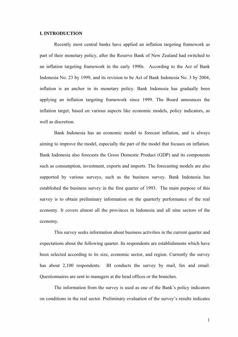
I. INTRODUCTION

Recently most central banks have applied an inflation targeting framework as

part of their monetary policy, after the Reserve Bank of New Zealand had switched to

an inflation targeting framework in the early 1990s. According to the Act of Bank

Indonesia No. 23 by 1999, and its revision to be Act of Bank Indonesia No. 3 by 2004,

inflation is an anchor in its monetary policy. Bank Indonesia has gradually been

applying an inflation targeting framework since 1999. The Board announces the

inflation target, based on various aspects like economic models, policy indicators, as

well as discretion.

Bank Indonesia has an economic model to forecast inflation, and is always

aiming to improve the model, especially the part of the model that focuses on inflation.

Bank Indonesia also forecasts the Gross Domestic Product (GDP) and its components

such as consumption, investment, exports and imports. The forecasting models are also

supported by various surveys, such as the business survey. Bank Indonesia has

established the business survey in the first quarter of 1993. The main purpose of this

survey is to obtain preliminary information on the quarterly performance of the real

economy. It covers almost all the provinces in Indonesia and all nine sectors of the

economy.

This survey seeks information about business activities in the current quarter and

expectations about the following quarter. Its respondents are establishments which have

been selected according to its size, economic sector, and region. Currently the survey

has about 2,100 respondents. BI conducts the survey by mail, fax and email.

Questionnaires are sent to managers at the head offices or the branches.

The information from the survey is used as one of the Bank’s policy indicators

on conditions in the real sector. Preliminary evaluation of the survey’s results indicates

2

that the survey is relatively weak in predicting the general economy performance

(GDP), also in explaining conditions in the sectors. To improve the quality of the

survey, several revisions have been made to the questions and methodology.

This paper consists of 5 parts. Part I describes the background and objectives of

the research paper. Part II illustrates the BI Business Survey (including the advantages

and limitations) and policy indicators. Part III describes about some proposed

improvement of Business survey to support the policy indicators, continued by Part IV

which tests the results of improvement. Finally, Part V is the summary and conclusion

of this research.

II. BANK INDONESIA BUSINESS SURVEY AND POLICY INDICATORS

2.1 Bank Indonesia Business Survey

As the central bank of Indonesia, BI’s single task is maintaining the stability of

Rupiah, the domestic currency. To conduct this task, BI needs information, including

information on business activities in the real sector. Since this information is currently

available from external sources and with a time lag, BI conducts its own survey (the

Bank Indonesia Business Survey).

In Indonesia, the business survey is conducted by three institutions i.e. Bank

Indonesia, Statistics Indonesia (BPS) and Danareksa Research Institute (the private

sector). In other countries such as Australia, the surveys are conducted by numerous

private institutions with various coverage areas. In Japan, the survey is conducted by

Bank of Japan. However, generally the information requested in the survey quite similar

i.e. relates to judgments on recent trends, on current situation and on expectations for

near term developments of the main economic variables.

This part will review the business survey conducted by Bank Indonesia,

including its advantages and limitations.

3

2.1.1. General Information

Bank Indonesia has established the business survey in the 1st quarter 1993. The

survey is conducted by Bank Indonesia’s head office together with 30 branch offices

spread over 29 provinces. Since the 1st quarter 2002 BI and Statistics Indonesia (BPS)

work together in doing this survey due to the harmonisation program initiate by OECD

and ADB.

Coverage

The BI business survey collects qualitative information on the comparison

between business activity in current quarter and previous quarter (realization) and

between current quarter and the next quarter (forecasting).

This survey covers nine (9) economic sectors in GDP with 7 types of

questionnaire designed for those sectors i.e.:

- Agriculture, Forestry and Fishery;

- Manufacturing, Mining and Quarrying;

- Electricity, Gas and Water Supply;

- Construction;

- Trade, Hotel and Restaurant;

- Transport and Communication;

- Financial, Rentals and Business Services; and Services.

. The information available in the survey is as follows:

- General Information;

- Business Activity (i.e. productions, capacity & business activity, labor usage,

business situation, selling prices/tariff/interest rate, financial condition and credit

access);

- Investment (actual and expectation);

4

- Others (expectation of inflation).

Questions are formulated as multiple choices, requesting answers of type “increase”,

“unchanged” or “decrease”. Questionnaires are filled by top managers, as they are better

capable of answering questions without referring to accounts, and able to convey future

anticipation of business evolution.

Sampling Method

The sampling method used in the survey is the stratified purposive sampling

technique. The respondents are stratified by the size (such as the number of employees

and production), region and economic sector. Currently around 2,100 companies

participate in the survey.

Processing Method

In processing the data, BI applies a Net Balance (NB) Method, which is

calculating the differences between the percentage number of respondent answering

“increase” and those who answer “decrease”, and left out those who answer “remain the

same”. If the results are:

(1) Positive Net Balance: expansion

(2) Negative Net Balance: contraction

(3) Zero Net Balance: stable

Bank Indonesia also use Weighted Net Balance (WNB) Method to calculate the single

business activity, in which the net balance in every sector is multiply with its own

weight – based on their share in GDP. The single score index is the sum up of WNB.

Release

The survey is released in a quarterly basis. When publishing the survey result,

Bank Indonesia head office (Directorate of Economic and Monetary Statistics) releases

5

on a nationwide basis. The head office’s report is based on the survey conducted by

head office and other branches.

However the individual branches could also release the survey results of the

companies within the region it covers. The difference between the business survey on a

nationwide basis released by the head office and surveys released by individual

branches is the samples. The branches survey include some respondents that are not

included in that of the nationwide-based (such as "local establishments of large

companies") in order to reflect the economic structure of each region.

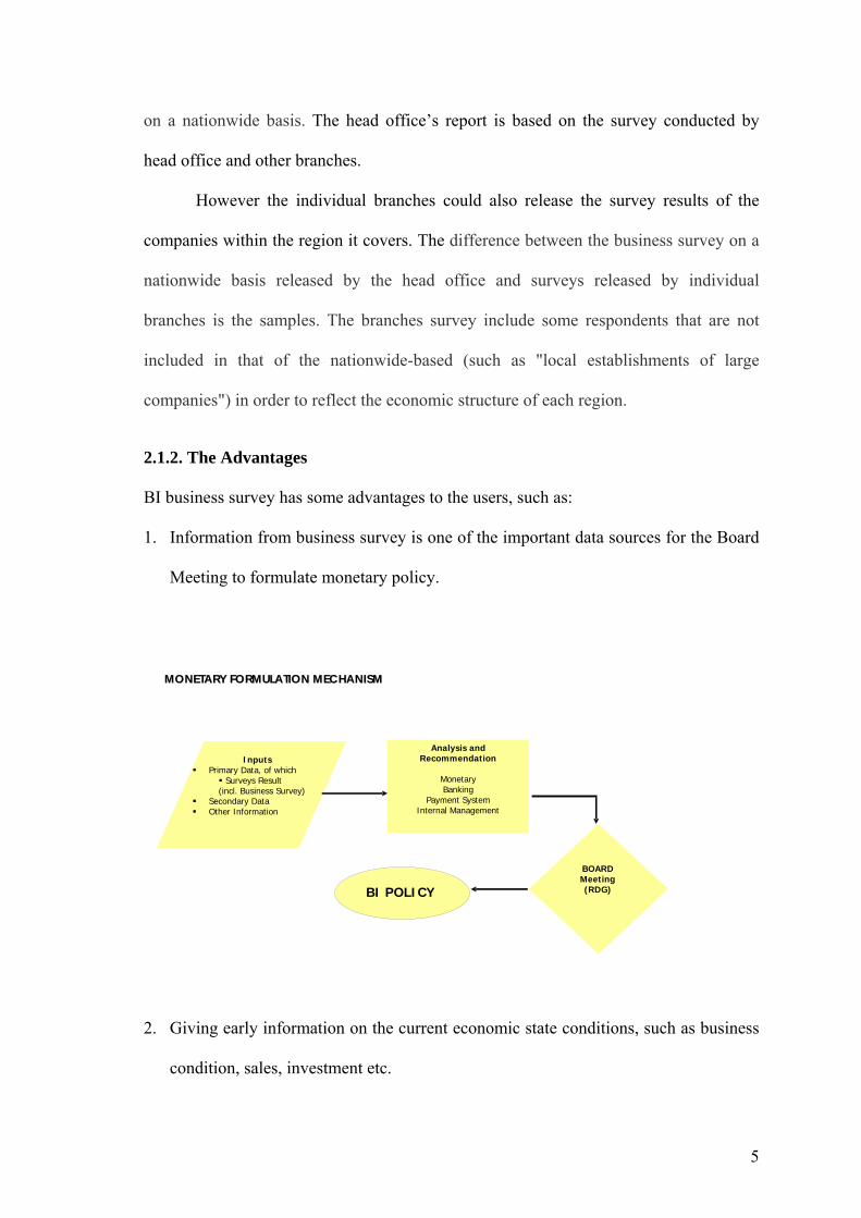
2.1.2. The Advantages

BI business survey has some advantages to the users, such as:

1. Information from business survey is one of the important data sources for the Board

Meeting to formulate monetary policy.

2. Giving early information on the current economic state conditions, such as business

condition, sales, investment etc.

6 6

MONETARY FORMULATION MECHANISMMONETARY FORMULATION MECHANISM

Inputs Primary Data, of which

Surveys Result(incl. Business Survey)

Secondary Data Other Information

Analysis and Recommendation

MonetaryBanking

Payment SystemInternal Management

BOARDMeeting (RDG)BI POLICY

6

3. Providing an indicator of expectations. This survey asks respondents about their

expectations, as well as about recent experiences. Information about expectations is

useful because companies’ views of future prospects can affect their current

behavior.

4. For the respondents, the survey result gives them input to formulate the plan to

expand their businesses.

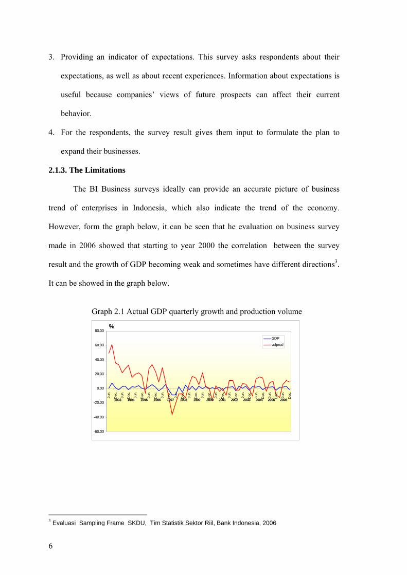
2.1.3. The Limitations

The BI Business surveys ideally can provide an accurate picture of business

trend of enterprises in Indonesia, which also indicate the trend of the economy.

However, form the graph below, it can be seen that he evaluation on business survey

made in 2006 showed that starting to year 2000 the correlation between the survey

result and the growth of GDP becoming weak and sometimes have different directions3.

It can be showed in the graph below.

Graph 2.1 Actual GDP quarterly growth and production volume

-60.00

-40.00

-20.00

0.00

20.00

40.00

60.00

80.00

Jun.

Dec

.

Jun.

Dec

.

Jun.

Dec

.

Jun.

Dec

.

Jun.

Dec

.

Jun.

Dec

.

Jun.

Dec

.

Jun.

Dec

.

Jun.

Dec

.

Jun.

Dec

.

Jun.

Dec

.

Jun.

Dec

.

Jun.

Dec

.

Jun.

Dec

.

GDP

volprod

1993 1994 1995 1996 1997 1998 1999 2000 2001 2002 2003 2004 2005 2006

%

3 Evaluasi Sampling Frame SKDU, Tim Statistik Sektor Riil, Bank Indonesia, 2006

7

We identify some limitations in BI business survey as follows:

(1) The Processing Method

a. No weighted

On calculating the Net Balance, companies are not weighted according to their sizes.

BI adopted the simple averages of the so-called "1 vote per company". In fact, the

companies’ size in the survey is in various range from small to big companies. Since

this is a qualitative survey, it can be misleading if conclusion are being drawn about

aggregate activity from the survey statistics. Changes in large companies will have

much larger impact on aggregate activity than a similar percentage change of a

small company. An example is in the case where the percentage of companies

answering increase similar with the companies answering decrease. The net balance

will be zero (0), which means that there is no change in the business activity. In fact,

it might be that most of the companies answering decrease are small companies

which have less impact to the economic conditions.

b. Using only one indicator

Bank Indonesia currently only has one indicator of business conditions in the

business survey, i.e. production volume. The National Australia Bank (NAB), for

example, takes the average of trading conditions, profitability and employment to

calculate general business conditions. BPS also uses some indicators to measure the

Tendency Business Index, i.e. revenue, production capacity, and employment

(number of employment, labor hours and wages).

(2) The Questionnaire

a. The degree of the qualitative answers

The degree of the qualitative answer in the questionnaire does not represent the

conditions when the companies experienced a small or moderate change. It is

8

potentially misleading. An investigation to the respondents of CBI’s Industrial

Trends Survey in the UK showed that the respondents have some range of output

variation that they regard as essentially “unchanged”, which termed as “the

indifference band”. The band could be in a range of 1% - 8%. 4 So that, in the case

of an upgrading the expectations from “unchanged” to “moderate increase” will

give different result in net balance method.

b. Consists of many questions

BI Business survey consists of lots of questions, which can be a burden for

respondents and possibly will cause them reluctant to respond the survey. Some of

the questions are designed to accommodate several interests, not only from the

Directorate of Economic and Monetary Statistics who conduct the survey, but also

from other directorates in BI. Moreover, since the survey is the joint survey with

Statistics of Indonesia (BPS) and must have harmonization with OECD, we have

added some more questions. The total number of question in the questionnaire is

nearly 50 questions. Actually, some of the questions are not related to the business

surveys, for example the questions regarding companies’ financial conditions and

credit access.

2.2. Policy Indicators

Both government and central bank concern to some economic indicators, such as

indicators of economic growth and indicator of inflation. Economic growth or Gross

Domestic Product (GDP) growth is very important to measure improvement of

economic. Therefore, governments usually want to improve their GDP growth.

Moreover, GDP is one of the tools to measure the wealthy level of country.

4 Quantifying Survey Data, Alastair Cunningham, Bank of England Quarterly Bulletin, August 1997.

9

Another important indicator is indicator of inflation, since inflation shows the

changes of price. Therefore, central bank needs to have the indicator of inflation to

picture the actual inflation. The main goal of almost all central banks is to achieve a low

and stable inflation. Some of them have already applied inflation targeting framework.

To support the inflation control, they need to get inflation indicator.

Both indicators are obtained by conducting the business survey as we mentioned

in the previous chapter. In this chapter, we divide two sub-chapters. The first is

indicator of economic growth to capture the flows of GDP growth and the second is

indicator of inflation.

2.2.1 Indicator of Economic Growth

Some countries have used some indicators from the survey to capture the flows

of GDP. In general, they have applied business activities as indicator of economic

growth or GDP growth. Bank Indonesia has business survey to support one of some

indicators that usually used by many economists as economic indicators.

One of the data that we gained from Bank Indonesia business survey is

production volume. The production volume has been applied as business activity that is

one of the indicators of economic growth. However, as noted earlier this indicator is

often misleading with real GDP growth.

Meanwhile, the Reserve Bank of Australia has a better economic indicator for

economic growth. They analyse various business surveys, e.g. the Quarterly Business

Survey from the National Australia Bank (NAB), the AIG survey, the ACCI-Westpac

survey and the Sensis survey. Each survey produces a business conditions index,

calculated as the average of trading conditions, profitability and employment. The RBA

then uses a principal component analysis to estimate an overall business conditions

indicator.

10

2.2.2 Indicator of Inflation

This indicator can help board of governor to make decision in monetary policy.

With supporting by forecasting model, inflation indicator will be helpful to capture the

flow of Consumer Price Index (CPI). Since the main goal of the central bank is to

control inflation, they really need this indicator to show that inflation target whether

achieved or not at current time.

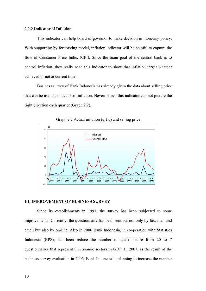
Business survey of Bank Indonesia has already given the data about selling price

that can be used as indicator of inflation. Nevertheless, this indicator can not picture the

right direction each quarter (Graph 2.2).

Graph 2.2 Actual inflation (q-t-q) and selling price

-10

0

10

20

30

40

50

2 3 4 1 2 3 4 1 2 3 4 1 2 3 4 1 2 3 4 1 2 3 4 1 2 3 4 1 2 3 4 1 2 3 4 1 2 3 4 1 2 3 4

InflationSelling Price

%

1993 1994 1995 1996 1997 1998 1999 2000 2001 2002 2003 2004 2005 2006

III. IMPROVEMENT OF BUSINESS SURVEY

Since its establishments in 1993, the survey has been subjected to some

improvements. Currently, the questionnaire has been sent out not only by fax, mail and

email but also by on-line. Also in 2006 Bank Indonesia, in cooperation with Statistics

Indonesia (BPS), has been reduce the number of questionnaire from 20 to 7

questionnaires that represent 9 economic sectors in GDP. In 2007, as the result of the

business survey evaluation in 2006, Bank Indonesia is planning to increase the number

11

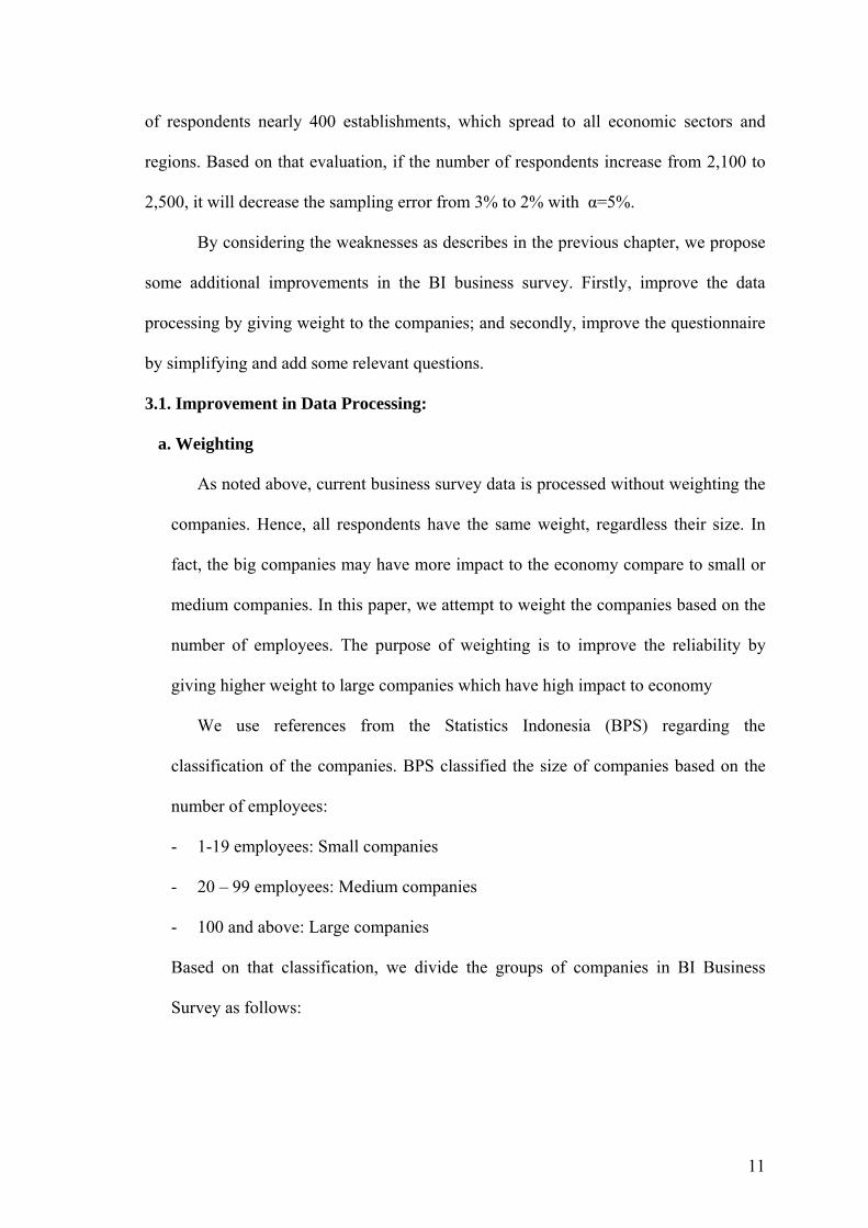
of respondents nearly 400 establishments, which spread to all economic sectors and

regions. Based on that evaluation, if the number of respondents increase from 2,100 to

2,500, it will decrease the sampling error from 3% to 2% with α=5%.

By considering the weaknesses as describes in the previous chapter, we propose

some additional improvements in the BI business survey. Firstly, improve the data

processing by giving weight to the companies; and secondly, improve the questionnaire

by simplifying and add some relevant questions.

3.1. Improvement in Data Processing:

a. Weighting

As noted above, current business survey data is processed without weighting the

companies. Hence, all respondents have the same weight, regardless their size. In

fact, the big companies may have more impact to the economy compare to small or

medium companies. In this paper, we attempt to weight the companies based on the

number of employees. The purpose of weighting is to improve the reliability by

giving higher weight to large companies which have high impact to economy

We use references from the Statistics Indonesia (BPS) regarding the

classification of the companies. BPS classified the size of companies based on the

number of employees:

- 1-19 employees: Small companies

- 20 – 99 employees: Medium companies

- 100 and above: Large companies

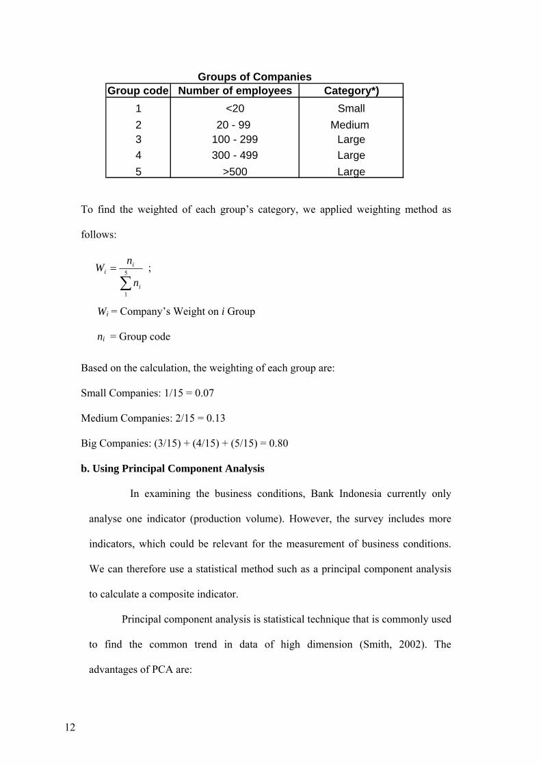
Based on that classification, we divide the groups of companies in BI Business

Survey as follows:

12

To find the weighted of each group’s category, we applied weighting method as

follows:

∑

= 5

1i

ii

n

nW ;

Wi = Company’s Weight on i Group

ni = Group code

Based on the calculation, the weighting of each group are:

Small Companies: 1/15 = 0.07

Medium Companies: 2/15 = 0.13

Big Companies: (3/15) + (4/15) + (5/15) = 0.80

b. Using Principal Component Analysis

In examining the business conditions, Bank Indonesia currently only

analyse one indicator (production volume). However, the survey includes more

indicators, which could be relevant for the measurement of business conditions.

We can therefore use a statistical method such as a principal component analysis

to calculate a composite indicator.

Principal component analysis is statistical technique that is commonly used

to find the common trend in data of high dimension (Smith, 2002). The

advantages of PCA are:

Group code Number of employees Category*)1 <20 Small2 20 - 99 Medium 3 100 - 299 Large4 300 - 499 Large5 >500 Large

Groups of Companies

13

a. If the data patterns are to be hard to find in high dimension data and the

graphical representation is not available, PCA will be a powerful tool in

analyzing the data.

b. If we compress the data, for instance, by reducing the number of dimensions,

we will be not lose much information, because we already have found the

patterns in the data.

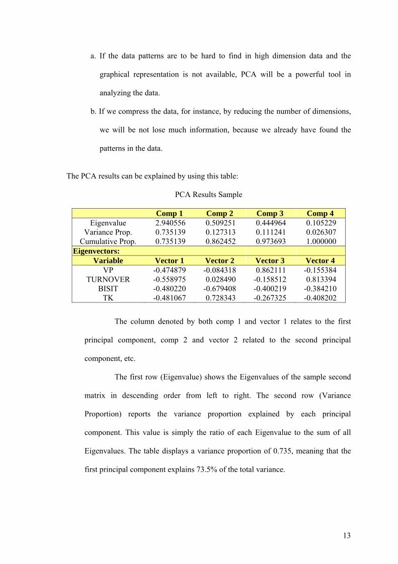
The PCA results can be explained by using this table:

PCA Results Sample

Comp 1 Comp 2 Comp 3 Comp 4 Eigenvalue 2.940556 0.509251 0.444964 0.105229

Variance Prop. 0.735139 0.127313 0.111241 0.026307 Cumulative Prop. 0.735139 0.862452 0.973693 1.000000

Eigenvectors: Variable Vector 1 Vector 2 Vector 3 Vector 4

VP -0.474879 -0.084318 0.862111 -0.155384 TURNOVER -0.558975 0.028490 -0.158512 0.813394

BISIT -0.480220 -0.679408 -0.400219 -0.384210 TK -0.481067 0.728343 -0.267325 -0.408202

The column denoted by both comp 1 and vector 1 relates to the first

principal component, comp 2 and vector 2 related to the second principal

component, etc.

The first row (Eigenvalue) shows the Eigenvalues of the sample second

matrix in descending order from left to right. The second row (Variance

Proportion) reports the variance proportion explained by each principal

component. This value is simply the ratio of each Eigenvalue to the sum of all

Eigenvalues. The table displays a variance proportion of 0.735, meaning that the

first principal component explains 73.5% of the total variance.

14

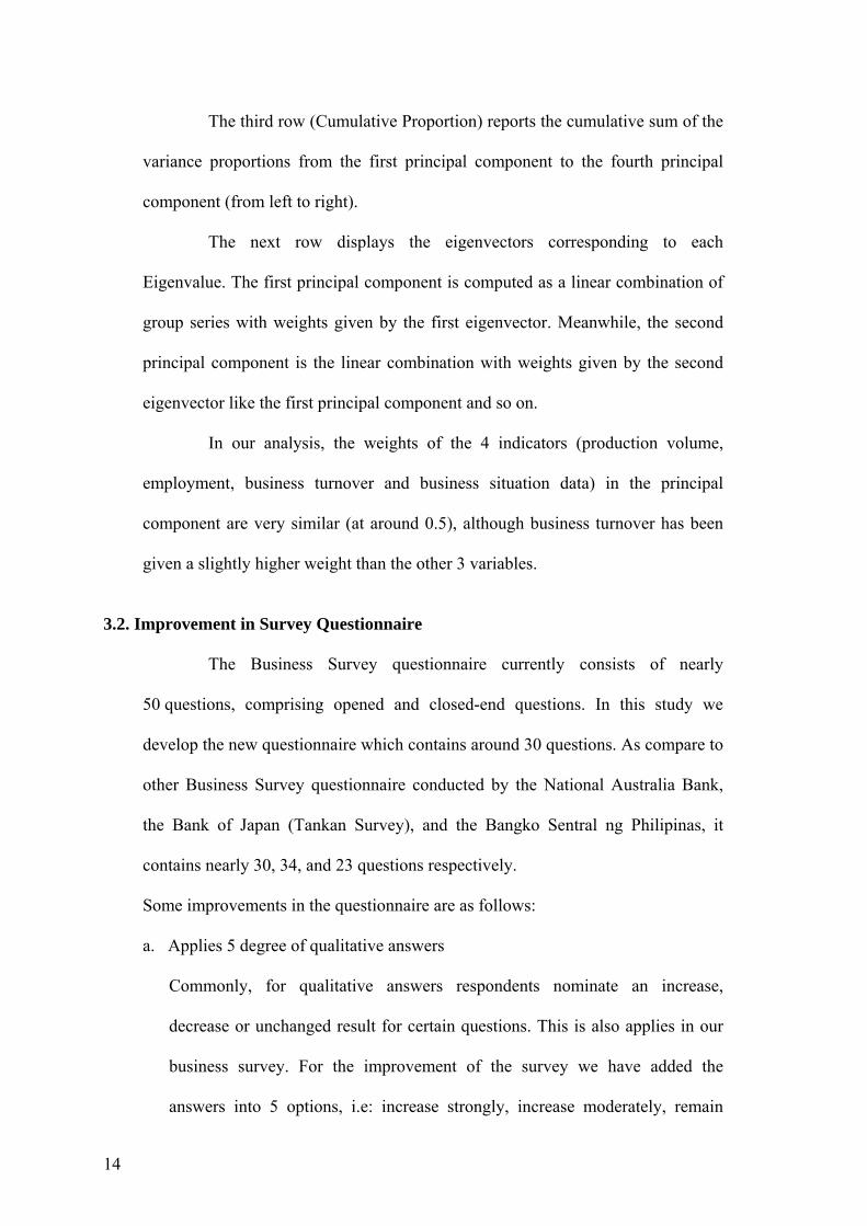
The third row (Cumulative Proportion) reports the cumulative sum of the

variance proportions from the first principal component to the fourth principal

component (from left to right).

The next row displays the eigenvectors corresponding to each

Eigenvalue. The first principal component is computed as a linear combination of

group series with weights given by the first eigenvector. Meanwhile, the second

principal component is the linear combination with weights given by the second

eigenvector like the first principal component and so on.

In our analysis, the weights of the 4 indicators (production volume,

employment, business turnover and business situation data) in the principal

component are very similar (at around 0.5), although business turnover has been

given a slightly higher weight than the other 3 variables.

3.2. Improvement in Survey Questionnaire

The Business Survey questionnaire currently consists of nearly

50 questions, comprising opened and closed-end questions. In this study we

develop the new questionnaire which contains around 30 questions. As compare to

other Business Survey questionnaire conducted by the National Australia Bank,

the Bank of Japan (Tankan Survey), and the Bangko Sentral ng Philipinas, it

contains nearly 30, 34, and 23 questions respectively.

Some improvements in the questionnaire are as follows:

a. Applies 5 degree of qualitative answers

Commonly, for qualitative answers respondents nominate an increase,

decrease or unchanged result for certain questions. This is also applies in our

business survey. For the improvement of the survey we have added the

answers into 5 options, i.e: increase strongly, increase moderately, remain

15

steady, decline moderately and decline strongly. These options are applied to

reduce the possibility that the respondents answer the same/remain steady,

even if the companies faced slightly increase/slightly decrease in the business.

b. Exclude some questions.

Based on our experiences, the respondents frequently leave opened-end

questions blank. However, if we give the choices for the answer they will fill

the questions. We also exclude some questions that have not relation to the

business survey. For instance in the Financial Part we take out the questions

regarding interest rate, credit access etc.

c. Include some new questions related to policy indicators.

From our business survey, we already have information about volume ordered

by foreign countries, but this is not specifically capture the export volume at

the current moment. Firms can export anytime depending on the order time

exactly. Meanwhile, we already have information about investment, but the

question about investment is only asked in each semester not each quarter like

other data. We can learn from ABS (Australian Bureau of Statistics) that

conducted Capital Expenditure Survey in quarterly basis. Their question about

investment is investment growth for a year in current quarter.

For that reason, some questions that we need to add in the new questionnaire

are as follows:

- For GDP indicators we add questions regarding export, import and

investment.

- For inflation indicators we add questions regarding labor cost, raw material

cost and overhead cost.

16

With the new questionnaire, we have conducted a small survey with 38

respondents located in Jakarta. Based on the interview with some respondents, we

have information as follows:

a. In qualitative answer, practically the respondents have a range for the answer

“remain steady/unchanged” i.e. between 1-5%.

b. They prefer closed-end questions rather than opened-end questions.

In processing the data from the new questionnaire, we weight both for the size of

companies and the degree of answers. The weighting for company size is similar

with previous improvement. In weighting the answers we use the method as follows:

- increase strongly = 2

- increase moderately = 1

- remain steady = 0

- decline moderately = -1

- decline strongly = -2

Then we used Net Balance method to calculate each variable.

IV. INVESTIGATING THE IMPROVEMENTS

In this chapter, we look at the results of the improvements, as discusses above. Firstly,

improvement is to formulate the weighted based on the size of firms. Secondly, we

develop the new questionnaire by changing the multiple choices answer and by

changing the number of question. Both of them improve the result that we need to solve

the problem.

4.1. Results of processing data improvement

In this part, we find that the improvement by applying weighted value shows

different result. For comparison, we analyze the indicator of GDP using production

17

volume in business survey. The indicator looks far from the actual GDP. Applying five

years period quarterly data (2003-2007), the direction of indicator shows different trend

in some quarters.

Graph 4.1 The plot of GDP quarterly and GDP indicator (production volume)

0

0.005

0.01

0.015

0.02

0.025

0.03

0.035

0.04Ja

n-03

Apr-

03

Jul-0

3

Oct

-03

Jan-

04

Apr-

04

Jul-0

4

Oct

-04

Jan-

05

Apr-

05

Jul-0

5

Oct

-05

Jan-

06

Apr-

06

Jul-0

6

Oct

-06

Jan-

07

Apr-

07

VolProd

GDP Growth

In empirical results by Granger Causality (table 4.1), we found that the null

hypothesis is that indicator denoted by VOP (production volume) does not Granger-

cause GDP quarterly (GDPQ) in the first regression. The test result stated that the

probability is 0.104 therefore we should accept the null hypothesis. It means indicator

does not Granger causing GDP quarterly. Similarly, in second regression, the test result

said that the probability is 0.15 therefore we accept the null hypothesis that GDP

quarterly does not Granger causing indicator.

Table 4.1 Granger Causality Test Null Hypothesis F-Statistic Probability

VOP does not Granger Cause GDPQ 3.01942 0.10421 GDPQ does not Granger Cause VOP 2.26180 0.15482

Therefore, we can conclude that indicator does not Granger cause GDP growth

and vice versa. This result proves that production volume is not good enough to be

18

indicator of GDP. By the correlation test, we got the correlation coefficient 0.14

meaning correlation between two variables can explain around 14%.

Furthermore, we apply a PCA (principal component analysis) to our additional

indicators (production volume, employment, turnover, and business situation) to get a

broader measure of business conditions.

Table 4.2 reports that production volume, employment, turnover, and business

situation have very similar weights in the principal component and that they all move in

the same direction as the business cycle. The first principal component explains 73 per

cent of the variation in our data panel

Table 4.2 PCA Results

Comp 1 Comp 2 Comp 3 Comp 4 Eigenvalue 2.930944 0.856394 0.176444 0.036219

Variance Prop. 0.732736 0.214098 0.044111 0.009055 Cumulative Prop. 0.732736 0.946834 0.990945 1.000000

Eigenvectors: Variable Vector 1 Vector 2 Vector 3 Vector 4

TK -0.375092 0.819724 -0.196182 0.385839 TURNOVER -0.566997 0.164020 0.281400 -0.756588

VP -0.506183 -0.416236 -0.755287 0.008189 BS -0.530659 -0.357628 0.558451 0.527860

The first principal component (PC1) can now be compared with the GDP. As

shown in Graph 4.2, the new indicator seems to have a closer correlation with GDP than

the previous measure.

19

Graph 4.2 Indicator of GDP denoted by PCA1 and quarterly GDP actual

0

0.005

0.01

0.015

0.02

0.025

0.03

0.035

0.04

Jan-

03

Apr-

03

Jul-0

3

Oct

-03

Jan-

04

Apr-

04

Jul-0

4

Oct

-04

Jan-

05

Apr-

05

Jul-0

5

Oct

-05

Jan-

06

Apr-

06

Jul-0

6

Oct

-06

Jan-

07

Apr-

07

PCA1

GDP Growth

Furthermore, in empirical results by Granger Causality (table 4.3), we have

found that the probability for the first hypothesis is 0.16, higher than 10%, therefore we

can accept the null hypothesis that indicator denoted by PCA1 doesn’t Granger cause

GDP quarterly. It means the indicator does not Granger cause GDP quarterly.

Meanwhile, we found in the test result that probability of second regression is 0.34,

therefore, we can accept the null hypothesis that GDP quarterly does not Granger causes

indicator. In conclusion, indicator does not Granger cause GDP growth and vice versa.

The correlation test results the coefficient between two variables is 0.13 meaning only

13% correlation both of them can be explained.

Table 4.3 Granger Causality Test Null Hypothesis F-Statistic Probability

PCA1 does not Granger Cause GDPQ 2.24527 0.16032 GDPQ does not Granger Cause PCA1 1.28690 0.34333

Additionally, we develop the indicator by weighting value based on respondent.

Applying both production volume and employment and similarly with previous

indicator, we used PCA (principal component analysis) methods to obtain composite

index as indicator for GDP.

20

The PCA result shown on table 4.4 shows that business situation, employment,

turn over and production volume all move in the same direction and that the first

principal component explains 74 per cent of the variation in our data panel.

Table 4.4 PCA Results Comp 1 Comp 2 Comp 3 Comp 4

Eigenvalue 2.956359 0.772262 0.182809 0.088569 Variance Prop. 0.739090 0.193066 0.045702 0.022142

Cumulative Prop. 0.739090 0.932155 0.977858 1.000000 Eigenvectors:

Variable Vector 1 Vector 2 Vector 3 Vector 4 GDPTURN -0.473061 0.626539 0.116262 0.608396 GDPVOL -0.541447 -0.104260 -0.819326 -0.157066 GDPLAB -0.421458 -0.758753 0.299055 0.396526 GDPBS -0.552650 0.144472 0.475136 -0.669292

We have the composite index from PCA denoted by PCW as a proxy for GDP.

Graph 4.3 shows that the new indicator have a closer correlation with GDP than the

previous indicator.

Graph 4.3 Indicator of GDP with weighted correspondent denoted by PCA2 and GDP

quarterly

0

0.005

0.01

0.015

0.02

0.025

0.03

0.035

0.04

Jan-

03

Apr-

03

Jul-0

3

Oct

-03

Jan-

04

Apr-

04

Jul-0

4

Oct

-04

Jan-

05

Apr-

05

Jul-0

5

Oct

-05

Jan-

06

Apr-

06

Jul-0

6

Oct

-06

Jan-

07

Apr-

07

PCA2

GDP Growth

Finally, we do Granger causality test (table 4.5) that the probability of the first

hypothesis is 0.09, so we can reject the null hypothesis. It means that indicator denoted

21

by PCA2 Granger cause GDP quarterly. Similarly, GDP quarterly does Granger cause

indicator, since the probability of second regression is 0.19, so we can accept the null

hypothesis saying GDP quarterly does not Granger cause indicator. Therefore we can

conclude that the direction between two variables is only in one way. However, the

correlation test shows that the coefficient correlation is only 0.29 meaning only around

30% correlation between two variables.

Table 4.5 Granger Causality Test Null Hypothesis F-Statistic Probability

PCA2 does not Granger Cause GDPQ 3.08340 0.09013 GDPQ does not Granger Cause PCA2 1.99716 0.19308

4.2. Result of Questionnaire Improvement

In this part, we will analyze the result of new questionnaire by observing the

graph. By comparing each indicator in business survey, previous survey and new

survey, we can obtain the difference methods with different result. Please noted that

when comparing the results particularly in quarter I-2007 and quarter II-2007, we use

the same respondents with our small survey to make it comparable.

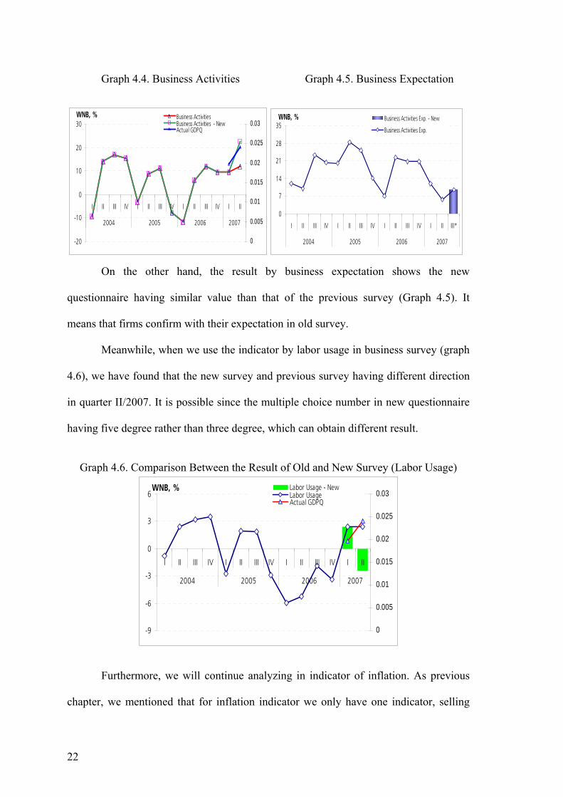
The business activities indicator as can be seen at Graph 4.4 shows that the

improvement with new survey achieves the higher value than that of old survey. This

situation shows that new survey resulting more optimistic in business activities in

quarter II/2007. Actual GDP quarterly is around 6% in quarter II/2007 in which this

growth is higher than prediction of some economic model.

22

Graph 4.4. Business Activities Graph 4.5. Business Expectation

-20

-10

0

10

20

30

I II III IV I II III IV I II III IV I II

2004 2005 2006 2007

0

0.005

0.01

0.015

0.02

0.025

0.03Business ActivitiesBusiness Activities - NewActual GDPQ

WNB, %

0

7

14

21

28

35

I II III IV I II III IV I II III IV I II III*

2004 2005 2006 2007

Business Activities Exp. - New

Business Activities Exp.

WNB, %

On the other hand, the result by business expectation shows the new

questionnaire having similar value than that of the previous survey (Graph 4.5). It

means that firms confirm with their expectation in old survey.

Meanwhile, when we use the indicator by labor usage in business survey (graph

4.6), we have found that the new survey and previous survey having different direction

in quarter II/2007. It is possible since the multiple choice number in new questionnaire

having five degree rather than three degree, which can obtain different result.

Graph 4.6. Comparison Between the Result of Old and New Survey (Labor Usage)

-9

-6

-3

0

3

6

I II III IV I II III IV I II III IV I II

2004 2005 2006 2007

0

0.005

0.01

0.015

0.02

0.025

0.03Labor Usage - NewLabor UsageActual GDPQ

WNB, %

Furthermore, we will continue analyzing in indicator of inflation. As previous

chapter, we mentioned that for inflation indicator we only have one indicator, selling

23

price, in previous questionnaire. Firstly, we will compare the selling price indicator of

inflation in old survey and new survey. Selling price indicator from previous survey as

shown in graph 4.7 tends to stable in quarter II/2007 compare with quarter I/2007.

Otherwise, new survey obtains different trend saying it increase in quarter II/2007

compare with the previous quarter.

Graph 4.7. Selling Price Graph 4.8. Selling Price Expectation

-10

0

10

20

30

40

I II III IV I II III IV I II III IV I II

2004 2005 2006 20070

0.5

1

1.5

2

2.5Selling Prices Selling Prices - NewInflasi q-t-q

WNB, %

-10

0

10

20

30

40

50

I II III IV I II III IV I II III IV I II III*

2004 2005 2006 2007

Selling Prices Exp.

Selling Prices Exp. - New

WNB, %

Moreover, graph 4.8 contains indicator of inflation expectation by selling price

expectation. It seems that the graph has similar trend between old survey and new

survey, though the new survey has higher number compare with the old survey.

The results in both graph 4.7 and graph 4.8 prove that improvement in new

questionnaire will obtain different result. Therefore, if we continue to apply new

questionnaire, hopefully we will get better result, since the previous inflation indicator

often in wrong direction.

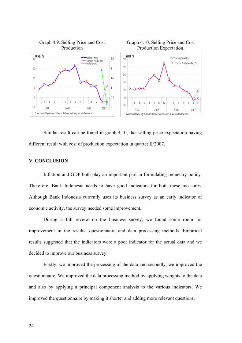
Furthermore, we extent to analyze the applying of some inflation indicator not

only selling price, but also overhead cost and labor cost. All indicators represented cost

denoted by cost production. In graph 4.9 the selling price indicator compares with cost

of production shows different direction in quarter II/2007 compare with the previous

quarter.

24

Graph 4.9. Selling Price and Cost Production

Graph 4.10. Selling Price and Cost Production Expectation.

-10

0

10

20

30

40

I II III IV I II III IV I II III IV I II

2004 2005 2006 2007 0

0.5

1

1.5

2

2.5Selling Prices Cost of Production *)Inflasi q-t-q

WNB, %

*) was counted by average method o f the labor, stationary and over head cost

-10

0

10

20

30

40

50

I II III IV I II III IV I II III IV I II III*

2004 2005 2006 2007

Selling Prices Exp.

Cost of Production Exp. *)

WNB, %

*) was counted by average method o f the labor exp, stationary exp. and over head exp. cost

Similar result can be found in graph 4.10, that selling price expectation having

different result with cost of production expectation in quarter II/2007.

V. CONCLUSION

Inflation and GDP both play an important part in formulating monetary policy.

Therefore, Bank Indonesia needs to have good indicators for both these measures.

Although Bank Indonesia currently uses its business survey as an early indicator of

economic activity, the survey needed some improvement.

During a full review on the business survey, we found some room for

improvement in the results, questionnaire and data processing methods. Empirical

results suggested that the indicators were a poor indicator for the actual data and we

decided to improve our business survey.

Firstly, we improved the processing of the data and secondly, we improved the

questionnaire. We improved the data processing method by applying weights to the data

and also by applying a principal component analysis to the various indicators. We

improved the questionnaire by making it shorter and adding more relevant questions.

25

The new weighted data, based on the new questionnaire and principal

component analysis, are giving different results than the current business survey. This

could be attributed to the limited sample and we will continue to evaluate the new

survey results as we receive more data.

REFERENCES

Aylmer, Chris and Gill, Troy (2003), “Business Survey and Economic Activity”,

Research Discussion Paper 2003-01, Economic Analysis Department, Reserve

Bank of Australia, February 2003.

Boivin, J. and S. Ng (2005), “Understanding and Comparing Factor Based Forecast”,

International Journal of Central Banking, 1, 117-151.

Carlson, John A., and Parkin, Michael (1975), “Inflation Expectation”, Economica,

New Series, Vol.42, No.166, pp.123-138.

Cunningham, Alastair (1997), “Quantifying Survey Data”, Bank of England Quarterly

Bulletin: August 1997.

Henzel, Steffen, and Wollmershauser, Timo (2005),”Quantifying Inflation Expectations

with the Carlson-Parkin Method”, Journal of Business Cycle Measurement and

Analysis, Vol.2, No.3, pp.321-371

Hofmann, Boris (2006), “Do Monetary Indicators (still) Predict Euro Area Inflation?”,

Discussion Paper Series 1: Economic Studies No 18/2006, Deutsche

Bundesbank.

Pesaran, M. Hashem, and Weale, Martin (2005),”Survey Expectations”, prepared for

inclusion in the Handbook of Economic Forecasting, North Holland.

Roberts, Ivan and Simon, John (2001), “What Do Sentiment Surveys Measure?”,

Research Discussion Paper 2001-09, Economic Research, Reserve Bank of

Australia, November 2001.

26

Stock, J. and M. Watson (2002b), “Forecasting Using Principal Component from a

Large Number of Predictors”, Journal of the American Statistical Association

97, 1167-1179.

Stock, James H (2004), “Forecasting with Many Predictors“, Department of Economic,

Hardvard University, NBER, August 2004.

Smith, Linday I (2002), “A Tutorial on Principal Component Analysis”, February 2002

Tim Statistik Sektor Riil (2006), “Evaluasi Sampling Frame SKDU”, Direktorat

Statistik Ekonomi dan Moneter, Bank Indonesia.