SEMINAR NASIONAL

METODE KUANTITATIF

2017

PROSIDING

Seminar Nasional

Metode Kuantitatif 2017

ISBN No. 978-602-98559-3-7

Editor :

Prof. Mustofa Usman, Ph.D

Dra. Wamiliana, M.A., Ph.D.

Layout & Design :

Shela Malinda Tampubolon

Alamat :

Fakultas Matematika dan Ilmu Pengetahuan Alam

Universitas Lampung, Bandar Lampung

Jl. Prof. Dr. Sumantri Brojonegoro No. 1 Bandar Lampung

Telp. 0721-701609/Fax. 0721-702767

Penggunaan Matematika, Statistika, dan Komputer dalam Berbagai Disiplin Ilmu

untuk Mewujudkan Kemakmuran Bangsa

KATA SAMBUTAN

KETUA PELAKSANA

SEMINAR NASIONAL METODE KUANTITATIF 2017

Seminar Nasional Metode Kuantitatif 2017 diselenggarakan oleh Jurusan Matematika Fakultas Matematika

dan Ilmu Pengetahuan Alam (FMIPA) Universitas Lampung yang dilaksanakan pada tanggal 24 – 25

November 2017. Seminar terselenggara atas kerja sama Jurusan Matematika FMIPA, Lembaga Penelitian

dan Pengabdian Masyarakat (LPPM) Unila, dan Badan Pusat Statistik (BPS).

Peserta dari Seminar dihadiri lebih dari 160 peserta dari 11 institusi di Indonesia, diantaranya : Kementrian

Pendidikan dan Kebudayaan, Badan Pusat Statistik, Universitas Indonesia, Institut Teknologi Bandung,

Universitas Sriwijaya, Universitas Jember, Universitas Islam Negeri Sunan Gunung Djati, Universitas

Cendrawasih, Universitas Teknokrat Indonesia, Universitas Malahayati, dan Universitas Lampung. Dengan

jumlah artikel yang disajikan ada sebanyak 48 artikel hal ini merefleksikan pentingnya seminar nasional

metode kuantitatif dengan tema “pengunaan matematika, statistika dan computer dalam berbagai disiplin

ilmu untuk mewujudkan kemakmuran bangsa”.

Kami berharap seminar ini menjadi tempat untuk para dosen dan mahasiswa untuk berbagi pengalaman dan

membangun kerjasama antar ilmuan. Seminar semacam ini tentu mempunyai pengaruh yang positif pada

iklim akademik khususnya di Unila.

Atas nama panitia, kami mengucapkan banyak terima kasih kepada Rektor, ketua LPPM Unila, dan Dekan

FMIPA Unila serta ketua jurusan matematika FMIPA Unila dan semua panitia yang telah bekerja keras untuk

suksesnya penyelenggaraan seminar ini.

Dan semoga seminar ini dapat menjadi agenda tahunan bagi jurusan matematika FMIPA Unila`

Bandar Lampung, Desember 2017

Prof. Mustofa Usman,Ph.D

Ketua Pelaksana

DAFTAR ISI

KATA SAMBUTAN . .................................................................................................................. iii

KEPANITIAAN . .......................................................................................................................... iv

DAFTAR ISI . ............................................................................................................................... vi

Aplikasi Metode Analisis Homotopi (HAM) pada Sistem Persamaan Diferensial Parsial

Homogen (Fauzia Anisatul F, Suharsono S, dan Dorrah Aziz) . ................................................. 1

Simulasi Interaksi Angin Laut dan Bukit Barisan dalam Pembentukan

Pola Cuaca di Wilayah Sumatera Barat Menggunakan Model Wrf-Arw

(Achmad Raflie Pahlevi) . ............................................................................................................. 7

Penerapan Mekanisme Pertahanan Diri (Self-Defense) sebagai Upaya Strategi Pengurangan

Rasa Takut Terhadap Kejahatan (Studi Pada Kabupaten/Kota di Provinsi Lampung yang

Menduduki Peringkat Crime Rate Tertinggi) (Teuku Fahmi) ...................................................... 18

Tingkat Ketahanan Individu Mahasiswa Unila pada Aspek Soft Skill

(Pitojo Budiono, Feni Rosalia, dan Lilih Muflihah) ................................................................... 33

Metode Analisis Homotopi pada Sistem Persamaan Diferensial Parsial Linear Non Homogen

Orde Satu (Atika Faradilla dan Suharsono S) . ........................................................................... 44

Penerapan Neural Machine Translation Untuk Eksperimen Penerjemahan Secara Otomatis

pada Bahasa Lampung – Indonesia (Zaenal Abidin) ................................................................... 53

Ukuran Risiko Cre-Var (Insani Putri dan Khreshna I.A.Syuhada) . ........................................... 69

Penentuan Risiko Investasi dengan Momen Orde Tinggi V@R-Cv@R

(Marianik dan Khreshna I.A.Syuhada) ........................................................................................ 77

Simulasi Komputasi Aliran Panas pada Model Pengering Kabinet dengan Metode Beda

Hingga (Vivi Nur Utami, Tiryono Ruby, Subian Saidi, dan Amanto) . ....................................... 83

Segmentasi Wilayah Berdasarkan Derajat Kesehatan dengan Menggunakan Finite Mixture

Partial Least Square (Fimix-Pls) (Agustina Riyanti) ................................................................... 90

Representasi Operator Linier Dari Ruang Barisan Ke Ruang Barisan L 3/2

(Risky Aulia Ulfa, Muslim Ansori, Suharsono S, dan Agus Sutrisno) . ...................................... 99

Analisis Rangkaian Resistor, Induktor dan Kapasitor (RLC) dengan Metode Runge-Kutta Dan

Adams Bashforth Moulton (Yudandi K.A., Agus Sutrisno, Amanto, dan Dorrah Aziz) . ............. 110

Edited with the trial version of Foxit Advanced PDF Editor

To remove this notice, visit:www.foxitsoftware.com/shopping

Representasi Operator Linier dari Ruang Barisan Ke Ruang Barisan L 13/12

(Amanda Yona Ningtyas, Muslim Ansori, Subian Saidi, dan Amanto) . ...................................... 116

Desain Kontrol Model Suhu Ruangan (Zulfikar Fakhri Bismar dan Aang Nuryaman) ............. 126

Penerapan Logika Fuzzy pada Suara Tv Sebagai Alternative Menghemat Daya Listrik

(Agus Wantoro) . ........................................................................................................................... 135

Clustering Wilayah Lampung Berdasarkan Tingkat Kesejahteraan (Henida Widyatama) ......... 149

Pemanfaatan Sistem Informasi Geografis Untuk Valuasi Jasa Lingkungan Mangrove dalam

Penyakit Malaria di Provinsi Lampung (Imawan A.Q., Samsul Bakri, dan Dyah W.S.R.W.) ..... 156

Analisis Pengendalian Persediaan Dalam Mencapai Tingkat Produksi Crude Palm Oil (CPO)

yang Optimal di PT. Kresna Duta Agroindo Langling Merangin-Jambi

(Marcelly Widya W., Hery Wibowo, dan Estika Devi Erinda) ................................................... 171

Analisis Cluster Data Longitudinal pada Pengelompokan Daerah Berdasarkan Indikator IPM

di Jawa Barat (A.S Awalluddin dan I. Taufik) . ............................................................................. 187

Indek Pembangunan Manusia dan Faktor Yang Mempengaruhinya di Daerah Perkotaan

Provinsi Lampung (Ahmad Rifa'i dan Hartono) .......................................................................... 195

Parameter Estimation Of Bernoulli Distribution Using Maximum Likelihood and Bayesian

Methods (Nurmaita Hamsyiah, Khoirin Nisa, dan Warsono) ..................................................... 214

Proses Pengamanan Data Menggunakan Kombinasi Metode Kriptografi Data Encryption

Standard dan Steganografi End Of File(Dedi Darwis, Wamiliana, dan Akmal Junaidi) . ........... 228

Bayesian Inference of Poisson Distribution Using Conjugate A

and Non-Informative Prior (Misgiyati, Khoirin Nisa, dan Warsono) . ....................................... 241

Analisis Klasifikasi Menggunakan Metode Regresi Logistik Ordinal dan Klasifikasi Naϊve

Bayes pada Data Alumni Unila Tahun 2016 (Shintia F., Rudi Ruswandi, dan Subian Saidi) . ... 251

Analisis Model Markov Switching Autoregressive (MSAR) pada Data Time Series

(Aulianda Prasyanti, Mustofa Usman, dan Dorrah Aziz) . ......................................................... 263

Perbandingan Metode Adams Bashforth-Moulton dan Metode Milne-Simpson dalam

Penyelesaian Persamaan Diferensial Euler Orde-8

(Faranika Latip., Dorrah Aziz, dan Suharsono S) . ....................................................................... 278

Pengembangan Ekowisata dengan Memanfaatkan Media Sosial untuk Mengukur Selera Calon

Konsumen (Gustafika Maulana, Gunardi Djoko Winarso, dan Samsul Bakri) . ........................ 293

Diagonalisasi Secara Uniter Matriks Hermite dan Aplikasinya pada Pengamanan Pesan

Rahasia (Abdurrois, Dorrah Aziz, dan Aang Nuryaman) . ........................................................... 308

Edited with the trial version of Foxit Advanced PDF Editor

To remove this notice, visit:www.foxitsoftware.com/shopping

Pembandingan Metode Runge-Kutta Orde 4 dan Metode Adam-Bashfort Moulton dalam

Penyelesaian Model Pertumbuhan Uang yang Diinvestasikan

(Intan Puspitasari, Agus Sutrisno, Tiryono Ruby, dan Muslim Ansori) . ................................... 328

Menyelesaikan Persamaan Diferensial Linear Orde-N Non

Homogen dengan Fungsi Green

(Fathurrohman Al Ayubi, Dorrah Aziz, dan Muslim Ansori) ..................................................... 341

Penyelesaian Kata Ambigu pada Proses Pos Tagging Menggunakan Algoritma Hidden

Markov Model ( HMM ) (Agus Mulyanto, Yeni Agus Nurhuda, dan Nova Wiyanto) ................. 347

Sistem Temu Kembali Citra Daun Tumbuhan Menggunakan Metode Eigenface

(Supiyanto dan Samuel A. Mandowen) . ...................................................................................... 359

Efektivitas Model Problem Solving dalam Meningkatkan Kemampuan Berfikir Lancar

Mahasiswa pada Materi Ph Larutan (Ratu Betta Rudibyani) ....................................................... 368

The Optimal Bandwidth for Kernel Density Estimation of Skewed Distribution: A Case Study

on Survival Data of Cancer Patients (Netti Herawati, Khoirin Nisa, dan Eri Setiawan) .......... 380

Karakteristik Larutan Kimia Di Dalam Air Dengan Menggunakan

Sistem Persamaan Linear (Titik Suparwati) . ................................................................................ 389

Bentuk Solusi Gelombang Berjalan Persamaan mKdV Yang Diperumum

(Notiragayu, Rudi Ruswandi, dan La Zakaria) . ......................................................................... 398

Pendugaan Blup Dan Eblup(Suatu Pendekatan Simulasi) (Nusyirwan) ...................................... 403

Edited with the trial version of Foxit Advanced PDF Editor

To remove this notice, visit:www.foxitsoftware.com/shopping

Prosiding Seminar Nasional Metode Kuantitatif 2017

ISBN No. 978-602-98559-3-7

214

Parameter Estimation of Bernoulli Distribution using

Maximum Likelihood and Bayesian Methods

Nurmaita Hamsyiah1), Khoirin Nisa1), &Warsono1) 1)Departmentof Mathematics, Faculty of Mathematics and Science, University of Lampung

Jl. Prof. Dr. Sumantri Brojonegoro No. 1 Bandar Lampung

Phone Number +62 721 701609 Fax +62 721 702767

E-mail: itamath98@gmail.com

ABSTRACT

The term parameter estimation refers to the process of using sample data to estimate the parameters of the

selected distribution.There are several methodsthat can be used to estimate distributionparameter(s).In this

paper,the maximum likelihood andBayesian methodsare usedfor estimating parameter ofBernoulli distribution,

i.e. , which isdefined asthe probability of success event for two possible outcomes.The maximum likelihood and

Bayesian estimators of Bernoulli parameter are derived,for the Bayesian estimator the Beta prior is used. The

analytical calculation shows that maximum likelihood estimator is unbiased while Bayesian estimator is

asymptotically unbiased. However, empirical analysis by Monte Carlo simulation shows that the mean square

errors (MSE) of the Bayesian estimatorare smaller than maximum likelihood estimator for large sample sizes.

Keywords: Bernoulli distribution, beta distribution, conjugate prior, parameter estimation.

1. PENDAHULUAN

Parameter estimation is a way to predict the characteristics of a population based on the sample taken. In general,

parameter estimation is classified into two types, namely point estimation and interval estimation. The point

estimation of a parameter is a value obtained from the sample and is used as a parameter estimator whose value

is unknown.

Several point estimation methods are used to calculate the estimator, such as moment method, maximum

likelihood method, and Bayesian method. The moment method predicts the parameters by equating the values of

sample moments to the population moment and solving the resulting equation system [1]. The maximum

likelihood (ML)methoduses differential calculus to determine the maximum of the likelihoodfunction to obtain

theparameters estimates. The Bayesianmethod differs from the traditional methods by introducing a frequency

function for the parameter being estimated namely prior distribution. The Bayesian method combines the prior

distribution and sample distribution. The prior distribution is the initial distribution that provides information

about the parameters. The sample distribution combined with the prior distribution provides a new distribution

i.e. the posterior distribution that expresses a degree of confidence regarding the location of the parameters after

the sample is observed [2].

Researches on parameter estimation using various methods of various distributions have been done, for example:

Bayesian estimation of exponential distribution [3], [4], ML and Bayesianestimations of Poisson distribution [5],

Bayesianestimation of Poisson-Exponential distribution [6], and Bayesianestimation of Rayleigh distribution [7].

The difference between the ML and the Bayesian methods is that the ML method considers that the parameter is

Prosiding Seminar Nasional Metode Kuantitatif 2017

ISBN No. 978-602-98559-3-7

215

an unknown quantity of fixed value and the inference is based only on the information in the sample; while the

Bayesian method considers the parameter as a variable that describes the initial knowledge of the parameters

before the observation is performed and expressed in a distribution called the prior distribution. After the

observation is performed, the information in the prior distribution is combined with the sample data information

through Bayesian theorem, and the result is expressed in a distribution form called the posterior distribution,

which further becomes the basis for inference in the Bayesian method [8].

The Bayesian method has advantages over other methods, one of which is the Bayesian method can be used for

drawing conclusions in complicated or extreme cases that cannot be handled by other methods, such as in

complex hierarchical models. In addition, if the prior information does not indicate complete and clear

information about the distribution of the prior, appropriate assumptions may be given to its distribution

characteristics. Thus, if the prior distribution can be determined, then a posterior distribution can be obtained

which may require mathematical computation [8].

This paper examines the parameter estimation of Bernoulli distribution using ML and Bayesianmethods. A

review of Bernoulli distribution and Beta distribution is presented in Section 2. The research methodologyis

described in Section 3. Section 4 provides the results and discussion. Finally, the conclusion is given in Section

5.

2. THEORETICAL FRAMEWORK

2.1 Bernoullli Distribution

Bernoulli distribution was introduced by Swiss mathematician,Jacob Bernoulli (1654-1705). It is the probability

distribution resulting from two outcomes or events in a given experiment, i.e. success ( ) and fail ( ),

with the probability of the success is θ and the probability of failure is .

Definition

A random variable is called a Bernoulli random variable (or is Bernoulli distributed) if and only if its

probability distribution is given by

( ) ( ) , for .

Proposition 1

Bernoulli distribution ( ) has mean and variance as follows:

and ( )

Proof :

The mean of Bernoulli random variable is

Prosiding Seminar Nasional Metode Kuantitatif 2017

ISBN No. 978-602-98559-3-7

216

( )

∑ ( )

∑ ( )

( ) ( )

The variance, i.e. ( ) ( ) , ( )- of Bernoulli distribution is obtained as follows:

( ) ∑ ( )

∑ ( )

∑ ( )

( ) ( )

Then,

( ) ( )

2.2. Beta Distribution

Definition

A random variable is called a betarandom variable with parametersa and b if the density function of is given

by

( ) {

( ) ( )

where ( )is betafunction defined as

( ) ∫ ( )

; (1)

Proposition 2

The beta function and gamma function is connected by

( ) ( ) ( )

( ) (2)

Proof :

( ) ( ) ∫

∫

Prosiding Seminar Nasional Metode Kuantitatif 2017

ISBN No. 978-602-98559-3-7

217

∫ ∫

Let ( ) and ( ) ( ),

( ) ( ) ∫ ∫( ) , ( )-

| ( )|

∫ ∫( ) , ( )-

∫ ∫ ( )

∫

∫ ( )

( ) ( )

Then,

( ) ( ) ( )

( )

Proposisi 3

The mean and variance of beta distribution with parametersaandbare

and

( )( )

Proof :

The proposition can be proved by using the moment ofbeta distribution as follows:

( )

( )∫ ( )

( )∫ ( ) ( )

From equations (1) and (2) we obtain

( ) ( )

( )

( ) ( )

( )

( ) ( )

( )

Prosiding Seminar Nasional Metode Kuantitatif 2017

ISBN No. 978-602-98559-3-7

218

( ) ( )

( ) ( )

( ) ( )

( ) ( )

( )) ( ) (3)

Thus the mean and variance of beta distribution will be obtained by substituting and to equation (3),

then

( ) ( ) ( ) ( )

( )) ( )

( ) ( )

( ) ( )) ( )

and ( ) ( ) , ( )- .

Since

( ) ( ) ( )

( )) ( )

( ) ( ) ( )

( ) ( ) ( )

( ) ( ) ( )

( )( ) ( ) ( )

( )

( )( ) ,

then

( ) ( )

( )( ) .

/

( )

( )( )

( )

( )( ) ( )

( ) ( )

( ) ( )

( ) ( )

3. RESEARCH METHOD

The research method for estimating the parameter of Bernoulli distribution in this paper can be described as

follows. For ML estimation, the parameter estimation is done by differentiatingpartially the log of the likelihood

Prosiding Seminar Nasional Metode Kuantitatif 2017

ISBN No. 978-602-98559-3-7

219

function and equation it by zero,

( )

to obtain ML estimator( ). The second derivation assessment is performed to show that the resulted truly

maximize the likelihood function. For the Bayesian method, the parameter estimation is done through the

following steps:

1. Form the likelihood function of Bernoulli distribution as follows:

( | ) ∏ (( )| )

2. Calculate the joint probability distribution, which is obtained by multiplying the likelihood function and the

prior distribution,

( ) ( | ) ( )

3. Calculate the marginal probability distribution function,

( ) ∫ ( )

4. Calculatethe posterior distributionby dividing the joint probability distribution function by the marginal

function,

( | ) ( )

( )

The Bayesian parameter estimate of is then produced as the mean of the posterior distribution.

After the parameter estimate of θis obtained by MLE and Bayesian methods, the evaluation of the estimators is

performed by assessing their bias, variance, and mean square error.

4. RESULT AND DISCUSSION

4.1. The ML Estimator of the Bernoulli Distribution Parameter ( )

Let be Bernoulli distributed random sample with ( ), where ( ). The

probability function of is

( ) ( ) with * +

The likelihood function of Bernoulli distribution is given by

( ) ( )

∏ ( )

∏ ( )

Prosiding Seminar Nasional Metode Kuantitatif 2017

ISBN No. 978-602-98559-3-7

220

( ) ( ) ( )

∑ ( ) ∑

. (4)

The natural logarithm of the likelihood function is then

( ) [ ∑ ( ) ∑

]

∑ ( ) ∑

∑ ( ∑

) ( ) (5)

The ML estimate value of is obtained by differentiating equation (5)with respect to andequating the

differential result to zero, i.e.

( )

[∑

( ∑

) ( )]

∑

∑

( )∑

( ∑

)

∑

∑

∑

∑

then we obtain

∑

To show that is the value that maximizes the likelihood function ( ), it must be confirmed that the second

derivative of the likelihood function for = is negative:

( )

[∑

( ∑

) ( )]

∑

∑

( )

( ) ∑

( ∑

)

( )

∑

∑

∑

∑

( )

Prosiding Seminar Nasional Metode Kuantitatif 2017

ISBN No. 978-602-98559-3-7

221

∑

∑

( )

Since maximizes the likelihood function, we conclude that the ML estimator of is given by

∑

4.2. The Bayesian Estimator of the Bernoulli Distribution Parameter( )

To estimate using Bayesian method, it is necessary to choose the initial information of a parameter called the

prior distribution, denoted by π(θ), to be applied to the basis of the method namely the conditional probability. In

this paper, the prior selection for Bernoulli distribution refers to the formation of its likelihood function. From

equation (4) we have

( ) ∑ ( ) ∑

A distribution having probability function in the same form as the above expression is the beta distribution with

density function

( )

( ) ( )

where ∑ , ∑

, and

( )are factors requiredfor the density function tobe satisfied.

The prior distributionis combinedwith the sample distribution to produce a new distribution calledposterior

distributionand denoted by ( | ). Posterior distributionis obtained by dividing the joint density

distribution by the marginal distribution.

Joint probability density function of( )is given by:

( ) ( | ) ( )

∑ ( ) ∑

( ) ( )

( ) ∑

( ) ∑

(6)

and the marginal function of ( ) is obtained as follows:

( ) ∫ ( )

Using equation (6) we have

( ) ∫

( ) ∑

( ) ∑

Prosiding Seminar Nasional Metode Kuantitatif 2017

ISBN No. 978-602-98559-3-7

222

( )∫ ∑

( ) ∑

( ) ( ∑ ∑

) (7)

Then from equation (6) and (7) the posterior distribution can be written as follows:

( | ) ( )

( )

( ) ∑

( ) ∑

( ) ( ∑ ∑

)

∑

( )

∑

( ∑ ∑

)

(8)

The posterior distribution expressed in equation (8) is obviously following beta distribution also with

parameter ( ∑ )and( ∑

), or

( ∑ ∑

).

Since the prior and posterior distribution of Bernoulli follows the same distribution, i.e. the Beta distribution,

beta distribution is called as the conjugate prior of the Bernoulli distribution. The posterior mean is used as the

parameter estimate θ in Bayesian method. Using Proposition 2, the Bayesian estimator of parameter θ is obtained

as follows:

∑

∑ ∑

∑

4.3. Evaluation of the Estimators Properties

The parameter estimationof the Bernoulli distribution isobtained by the MLE and Bayesian methods yields

different estimates. The best estimator has to meet the following properties:

1. Unbiased

An estimator is called to be unbiased if its expected values is equal to the estimated parameter, i.e. is an

unbiased estimator of if ( ) .The bias of an estimator is then given by:

( ) ( ) (9)

Let are Bernoulli( ) random sample observations. Since

∑ is the ML estimator of ,

its expected value is as follows:

Prosiding Seminar Nasional Metode Kuantitatif 2017

ISBN No. 978-602-98559-3-7

223

( ) (

∑

)

(∑

)

∑ ( )

(10)

Since ( ) , is an unbiased estimator of .

Now consider the Bayesian estimator of i.e. ∑

. The expexted value of Bayesian estimator is given

by

( ) ( ∑

)

( ∑

)

[ ( ) (∑

)]

[ ( ) ∑ ( )

]

( ) (11)

Since ( ) , is an biased estimator of . The bias value of is:

( ) ( )

(12)

Although is an biased estimator of , it can be shown that is asymptotically unbiased.The proof is given as

follows:

( )

Prosiding Seminar Nasional Metode Kuantitatif 2017

ISBN No. 978-602-98559-3-7

224

(13)

Since ( ) , is an asymptotically unbiased estimator of .

2. Efficiency

The efficiency of an estimator is observed from its variance. The best parameter estimator is the one that has the

smallest variance. This is because the variance of an estimator is a measure of the spread of the estimator around

its mean.

The variance of ML estimator is:

( ) (

∑

)

(∑

)

∑ ( )

( )

( ) (14)

While the variance of the Bayesian estimator is given by:

( ) ( ∑

)

( ) ( ∑

)

( ) [ ( ) ∑ ( )

]

Since ( ) and ( ) ( ), we obtain

( )

( ) ( ) (15)

From equation (10), it is shown that the ML estimator is unbiased, whereas from equations (11) and (12) it is

shown that Bayesian estimator is biased. As a result, the efficiency of the two methods cannot be compared

because the efficiency of estimators applies to unbiased estimators.

Prosiding Seminar Nasional Metode Kuantitatif 2017

ISBN No. 978-602-98559-3-7

225

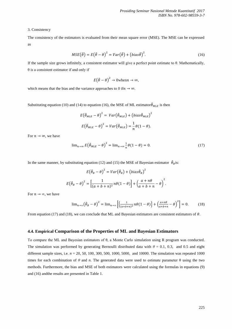
3. Consistency

The consistency of the estimators is evaluated from their mean square error (MSE). The MSE can be expressed

as

( ) ( ) ( ) ( )

(16)

If the sample size grows infinitely, a consistent estimator will give a perfect point estimate to θ. Mathematically,

θ is a consistent estimator if and only if

( ) when ,

which means that the bias and the variance approaches to 0 if .

Substituting equation (10) and (14) to equation (16), the MSE of ML estimator is then

( ) ( ) ( )

( ) ( )

( )

For , we have

( )

( ) (17)

In the same manner, by substituting equation (12) and (15) the MSE of Bayesian estimator is:

( ) ( ) ( )

( ) [

( ) ( )] (

)

For , we have

( ) [{

( ) ( )} .

/

] (18)

From equation (17) and (18), we can conclude that ML and Bayesian estimators are consistent estimators of .

4.4. Empirical Comparison of the Properties of ML and Bayesian Estimators

To compare the ML and Bayesian estimators of θ, a Monte Carlo simulation using R program was conducted.

The simulation was performed by generating Bernoulli distributed data with θ = 0.1, 0.3, and 0.5 and eight

different sample sizes, i.e. n = 20, 50, 100, 300, 500, 1000, 5000, and 10000. The simulation was repeated 1000

times for each combination of θ and n. The generated data were used to estimate parameter θ using the two

methods. Furthermore, the bias and MSE of both estimators were calculated using the formulas in equations (9)

and (16) andthe results are presented in Table 1.

Prosiding Seminar Nasional Metode Kuantitatif 2017

ISBN No. 978-602-98559-3-7

226

Table 1. The biasand MSEofML and Bayesian estimators of

N

Bias MSE

ML Bayesian

( ) ML

Bayesian

( )

0,1

20 0,001200 0,223084 0,031478 0,558149

50 0,002180 0,036602 0,015264 0,041740

100 0,000270 0,009328 0,007058 0,008843

300 0,000413 0,001075 0,001901 0,002906

500 0,000210 0,000364 0,001183 0,000551

1000 0,000195 0,000091 0,000503 0,000128

5000 0,000003 0,000003 0,000143 0,000004

10000 0,000114 0,000001 0,000184 0,000002

0,3

20 0,003100 0,536609 0,001652 0,493287

50 0,001300 0,090000 0,003113 0,142692

100 0,000630 0,021341 0,001583 0,067615

300 0,000003 0,002205 0,000327 0,002307

500 0,000312 0,000845 0,000111 0,000899

1000 0,000545 0,000207 0,000444 0,000217

5000 0,000384 0,000008 0,000403 0,000018

10000 0,000023 0,000002 0,000013 0,000004

0,5

20 0,001450 0,714234 0,023000 1,453419

50 0,002260 0,097036 0,011566 0,147045

100 0,003860 0,024341 0,008602 0,024833

300 0,000143 0,002856 0,001792 0,003374

500 0,000146 0,001004 0,001139 0,003040

1000 0,000432 0,000252 0,000929 0,000253

5000 0,000132 0,000009 0,000232 0,000056

10000 0,000066 0,000002 0,000016 0,000003

Table 1 shows the bias and MSE values of ML and Bayesian estimates for a successful probability of θ = 0.1, 0.3

and 0.5. From the table it can be seen ML estimator produces smaller biases than Bayesian estimates for finite

sample (i.e. n< 1000). However, when the sample size equal or larger than 1000 (i.e. 5000 and 10000, the

biasesof the Bayesian estimator are smaller than the ML estimator. Even though the bias values of ML estimates

changes inconsistently throughout the sample sizes, analytically it has been proved that ML estimator is an

unbiased estimator.This appears to be different from the bias values for Bayesian estimator. This is because for

all the considered success probabilitiesof the bias values become smaller whenthe sample size increases,

although analytically it is found that Bayesian estimatoris a biased estimator. As a result the efficiency of the two

estimators cannot be compared. Therefore, to compare the best estimators we use MSE of both estimators. This

is because MSE considers both the bias and variance values.

The MSE values of MLand Bayesian estimators that have been shown in Table 1 have similarities, i.e. the MSE

value decreases as the sample size increases and it closes to 0. Thus, both estimators are consistent estimators.

This also corresponds to the results obtained analytically. Based on the simulation results in this study, it can be

seen that for the larger sample sizes Bayesian estimatoris better than ML estimator. This is because the MSE

value of Bayesian estimator is smaller than the ML estimator. As shown in Table 1, when θ = 0.1, the MSE value

Prosiding Seminar Nasional Metode Kuantitatif 2017

ISBN No. 978-602-98559-3-7

227

of the Bayesian estimator is smaller than the ML estimator for n= 500, 1000, and 10000; and when θ = 0.3 and

0.5, the MSE values of the Bayesian estimator are smaller than the ML estimator for n = 1000, 5000, and 10000.

5. CONCLUSION

In this paper, we derived the ML and Bayesian estimator (using beta prior) of Bernoulli distribution parameter.

Analytically we show that the ML estimator is an unbiased estimator and Bayesian estimator is a biased

estimator for parameter θ. However, Bayesian estimator is asymptotically unbiased. Based on the simulation

result, both ML and Bayesian estimator are consistent estimators of θ because the two estimators satisfy the

property of consistency, i.e. ( ) whenn → ∞.The simulation result also shows that the

Bayesianestimator usingbeta prioris better than the MLE method for large sample sizes (n 1000).

REFERENCES

, - Bain, L.J. and Engelhardt, M. (1992).Introduction to Probability and Mathematical Statistics. Duxbury

Press, California.

, - Walpole, R.E dan Myers, R.H. (1995). Ilmu Peluang dan Statistika untuk Insinyur dan Ilmuwan. ITB,

Bandung.

, - Al-Kutubi H. S., Ibrahim N.A. (2009). Bayes Estimator for Exponential Distribution with Extensionof

Jeffery Prior Information. Malaysian Journal of MathematicalSciences. 3(2):297-313.

, - Nurlaila, D., Kusnandar D.,& Sulistianingsih, E. (2013). Perbandingan Metode Maximum Likelihood

Estimation (MLE) dan Metode Bayes dalam Pendugaan Parameter Distribusi Eksponensial. Buletin Ilmiah

Mat. Stat. dan Terapannya. 2(1):51-56.

, - Fikhri, M., Yanuar, F., & Yudiantri A. (2014). Pendugaan Parameter dari Distribusi Poisson dengan

Menggunakan Metode Maximum Likelihood Estimation (MLE) dan Metode Bayes. Jurnal Matematika

UNAND. 3(4):152-159.

, - Singh S. K., Singh, U., &Kumar, M. (2014). Estimation for the Parameter of Poisson-Exponential

Distribution under Bayesian Paradigm. Journal of Data Science.12:157-173.

, - Gupta, I. (2017). Bayesian and E-Bayesian Method of Estimation of Parameter of Rayleigh Distribution-A

Bayesian Approachunder Linex Loss Function. International Journal of Statistics and Systems.12(4):791-

796.

, - Box, G.E.P& Tiao, G.C. (1973). Bayesian Inference in Statistical Analysis. Addision-Wesley Publishing

Company, Philippines.