training course on flood risk assessment - icwrgc

UNESCO Office, JakartaJl. Galuh II No. 5Kebayoran BaruJakarta 12110 • IndonesiaTelephone: +62 (21) 739 9818Telefax: +62 (21) 7279 [email protected] • www.unesco.org/jakarta

International Centre for Water Resources and Global Change Federal Institute of Hydrology • P.O. Box 20025356002 Koblenz • GermanyTelephone: +49 (0)261/1306 - 5313 Telefax: +49 (0)261/1306 - [email protected] • www.waterandchange.org

United NationsEducational, Scientific and

Cultural Organization

International Centre for Water Resources and Global Changeunder the auspices of UNESCO

Training course on flood risk assessmentBiljana Radojevic and Pascal Breil




Table of content

Rationale 5

1 Introductory notions 7 1.1 Flood risk definition 7 1.2 Flood hazard definition 8 1.3 Vulnerability definition 8

2 Generalities 11 2.1 Inundation: a catchment process 11 2.2 Basic principles to mitigate inundation 12 2.3 Transient storage of flood peak volume 12 2.4 Opportunities for slowing down extreme runoff 12 2.5 Sources of flooding in urban systems 13 2.6 Why consider up- to downstream flooding management consequences 13 2.7 The effect of urbanization on the flood frequency 14 2.8 The effect of rural land use change on the flood frequency 14 2.9 Complex effects of urban development on flow extremes (flood and drought) 14 2.10 Where and how mitigate the flood hazard in a catchment? 15 2.11 Land vulnerability change along the stream network 16 2.12 Flood vulnerability change with time 16

3 Flood hazard modeling 17 3.1 Flow and flood predictability 17 3.2 Flood charcateristics 17 3.3 Intensity, duration and volume of floods 18 3.4 Sampling of flood flow characteristics 18 3.5 Sampling process of QCXd 19 3.6 Sampling process of VCXd 19 3.7 Illustration for a given flood event 19 3.8 Calculation of flood characteristics probability 20 3.9 Empirical Frequency formulae 20 3.10 Relation between F, F1 and T 20 3.11 Distribution of samples of VCX(d) as function of ln(T) 21 3.12 Introduction to QdF model and fitting 21 3.13 Probabilistic model formulae for QdF quantiles 22 3.14 QdF quantiles extrapolation to rare floods 22 3.15 QdF model representation 22 3.16 Methods for designing floods 23

4 | TABLE OF CONTENT

3.17 QdF based model method for designing a single period flood 23 3.18 Single period design floods and inundation limits 23 3.19 Inundation map limits for several HRP 23 3.20 What to do when no flow data exist at the place of interest? 24 3.21 QdF model scaling parameters D and QIX10 24 3.22 Predetermined sets of parameters of QdF model, VCX and QCX 24 3.23 How to size a detention hydraulic work 25

4 Vulnerability 27 4.1 How to express flood vulnerability? 27 4.2 An example of a vulnerability scale 27 4.3 Example of a vulnerability map 28 4.4 A Cost-Benefit approach of Vulnerability 29 4.5 Vulnerability considering high probability/low damage “VS” low probability/high

damage “flood events” 29 4.6 Integrated flood approach of the vulnerability-cost function 30

5 Flood risk mapping 31 5.1 Flood risk management rules using inundability approach 32 5.2 Conclusion on the inundability method implementation 32

6 List of Figures 35

Rationale

This training course sets out a general method for quantifying flood risk and the measures for risk mitigation. The method is general and does not depend on the flood model used. This course aims to give learners basic knowledge helping them to develop a feasibility study on flood risk management in a given area.

The first part of the course is dedicated to generalities and the presentation of a core concept to quantify flood risk.

The course then presents the probabilistic modeling of flood hazard and the qualification of vulnerability. This includes defining flood characteristics and their sampling procedure, building a probabilistic flood model using flow time series from regional analysis (or other sources for ungauged basins), using the model to design a projected flood event for a given return period, and finally from these data drawing up a method to design a dry dam for flood peak mitigation. The vulnerability assessment method is presented and tested from an existing flooded area. The objectives are to understand the flood characteristics

that are relevant to protect people and property, use the corresponding probabilistic models and the computer facilities available, calculate dry (or empty dam) storage capacity, and fit a regional model of flood hazard to generate prediction at ungauged basins.

This produces two maps: one for flood hazard (which can be made from a topographic map on the selected area prior to any complex hydraulic modeling, which is not within the scope of this course), and one for vulnerability of the area exposed to flooding.

The last part of the course focuses on flood risk map production and interpretation as well as on the work involved in appropriately locating empty dams, levees, and flooded areas. Calculating required storage capacities and the cost estimation of different scenarios and their expected effectiveness is also discussed. The objective is to train learners in the necessity of an iterative process of discussion and simulation to reach the most feasible and accepted solution for vulnerable communities and to prevent them from the consequences of flooding.

1 Introductory Notions

same numerical value have equal “significance” but this is often not the case… low probability / high consequence events are treated very differently to high probability / low consequence events” (Sayers et al. 2002).

· “Risk is the actual exposure of something of human value to a hazard and is often regarded as the combination of probability and loss” (Smith 1996).

· “Risk might be defined simply as the probability of the occurrence of an undesired event (but) be better described as the probability of a hazard contributing to a potential disaster… importantly, it involves consideration of vulnerability to the hazard” (Stenchion 1997).

· Risk is “Expected losses (of lives, persons injured, property damaged, and economic activity disrupted) due to a particular hazard for a given area and reference period. Based on mathematical calculations, risk is the product of hazard and vulnerability” (UN DHA).

The most common definition of risk used in flood management is that risk expresses the combination of flood hazard and flood vulnerability at a given location. In this case, exposure is implicit because the area of interest is the flooded area.

Flood risk increases when the flood intensity is high at a place where vulnerability is also high. However, both hazard and vulnerability have spatial variations. Flood risk can change considerably from one place to another in the flood-exposed area.

A simple way to interpret flood risk is then to subtract the vulnerability return period (VRP) from the hazard return period (HRP). The positive values indicate that

1.1 Flood risk definition

There are several definitions of risk in the literature: · Total risk = Impact of hazard ‘Elements at risk’

Vulnerability of elements at risk (Blong, 1996, citing UNESCO)

· “Risk is the probability of a loss, and this depends on three elements, hazard, vulnerability and exposure. If any of these three elements in risk increases or decreases, then risk increases or decreases respectively (Crichton, 1999).”

· Risk = Hazard × Vulnerability × Value (of the threatened area) / Preparedness (De La Cruz-Reyna, 1996).

· “Risk (i.e. ‘total risk’) means the expected number of lives lost, persons injured, damage to property and disruption of economic activity due to a particular natural phenomenon, and consequently the product of specific risk and elements at risk.” Total risk can be expressed in pseudo- mathematical form as:

· Total Risk = Hazard × Vulnerability × Elements at Risk – (as modified by Granger et al., 1999)

· Risk = Probability × Consequences (Helm, 1996)

· “Risk is a combination of the chance of a particular event, with the impact that the event would cause if it occurred. Risk therefore has two components – the chance (or probability) of an event occurring and the impact (or consequence) associated with that event. The consequence of an event may be either desirable or undesirable… In some, but not all cases, therefore a convenient single measure of the importance of a risk is given by: Risk = Probability × Consequences. […] Intuitively it may be assumed that risks with the

8 | INTRODUCTORY NOTIONS

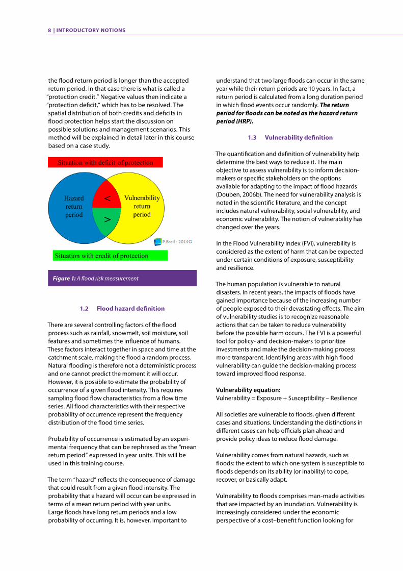
the flood return period is longer than the accepted return period. In that case there is what is called a

“protection credit.” Negative values then indicate a “protection deficit,” which has to be resolved. The spatial distribution of both credits and deficits in flood protection helps start the discussion on possible solutions and management scenarios. This method will be explained in detail later in this course based on a case study.

understand that two large floods can occur in the same year while their return periods are 10 years. In fact, a return period is calculated from a long duration period in which flood events occur randomly. The return period for floods can be noted as the hazard return period (HRP).

1.3 Vulnerability definition

The quantification and definition of vulnerability help determine the best ways to reduce it. The main objective to assess vulnerability is to inform decision- makers or specific stakeholders on the options available for adapting to the impact of flood hazards (Douben, 2006b). The need for vulnerability analysis is noted in the scientific literature, and the concept includes natural vulnerability, social vulnerability, and economic vulnerability. The notion of vulnerability has changed over the years.

In the Flood Vulnerability Index (FVI), vulnerability is considered as the extent of harm that can be expected under certain conditions of exposure, susceptibility and resilience.

The human population is vulnerable to natural disasters. In recent years, the impacts of floods have gained importance because of the increasing number of people exposed to their devastating effects. The aim of vulnerability studies is to recognize reasonable actions that can be taken to reduce vulnerability before the possible harm occurs. The FVI is a powerful tool for policy- and decision-makers to prioritize investments and make the decision-making process more transparent. Identifying areas with high flood vulnerability can guide the decision-making process toward improved flood response. Vulnerability equation:Vulnerability = Exposure + Susceptibility – Resilience

All societies are vulnerable to floods, given different cases and situations. Understanding the distinctions in different cases can help officials plan ahead and provide policy ideas to reduce flood damage.

Vulnerability comes from natural hazards, such as floods: the extent to which one system is susceptible to floods depends on its ability (or inability) to cope, recover, or basically adapt.

Vulnerability to floods comprises man-made activities that are impacted by an inundation. Vulnerability is increasingly considered under the economic perspective of a cost–benefit function looking for

Figure 1: A flood risk measurement

1.2 Flood hazard definition

There are several controlling factors of the flood process such as rainfall, snowmelt, soil moisture, soil features and sometimes the influence of humans. These factors interact together in space and time at the catchment scale, making the flood a random process. Natural flooding is therefore not a deterministic process and one cannot predict the moment it will occur. However, it is possible to estimate the probability of occurrence of a given flood intensity. This requires sampling flood flow characteristics from a flow time series. All flood characteristics with their respective probability of occurrence represent the frequency distribution of the flood time series.

Probability of occurrence is estimated by an experi-mental frequency that can be rephrased as the “mean return period” expressed in year units. This will be used in this training course.

The term “hazard” reflects the consequence of damage that could result from a given flood intensity. The probability that a hazard will occur can be expressed in terms of a mean return period with year units.Large floods have long return periods and a low probability of occurring. It is, however, important to

INTRODUCTORY NOTIONS | 9

decision criteria to build flood protection. Natural resources are now being considered using the approach of ecosystem services, but this is presently limited to research and demonstration. The cost- benefit approach remains difficult for implementation considering indirect side-effects of floods, which can, for example, disrupt transportation of goods between producers, suppliers, retailers, and consumers.

The choice that can be made is to assess the feasibility of implementing flood mitigation responses using popula-tion and market expectations in terms of a desirable return period of protection – noted VRP (vulnerability return period). This method has a very important advantage, developing an iterative process of dialogue between the actors concerned in the flooded area using an easy-to-share representation of vulnerability level.

2 Generalities

2.1 Inundation: a catchment process

Flood frequency analysis and model building or model calibration is based on the availability of the flow time series.

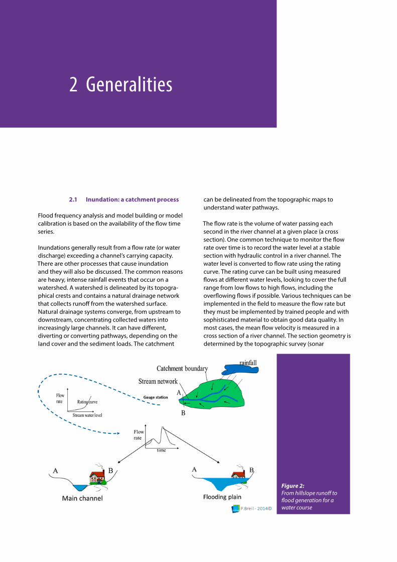
Inundations generally result from a flow rate (or water discharge) exceeding a channel’s carrying capacity. There are other processes that cause inundation and they will also be discussed. The common reasons are heavy, intense rainfall events that occur on a watershed. A watershed is delineated by its topogra-phical crests and contains a natural drainage network that collects runoff from the watershed surface. Natural drainage systems converge, from upstream to downstream, concentrating collected waters into increasingly large channels. It can have different, diverting or converting pathways, depending on the land cover and the sediment loads. The catchment

can be delineated from the topographic maps to understand water pathways.

The flow rate is the volume of water passing each second in the river channel at a given place (a cross section). One common technique to monitor the flow rate over time is to record the water level at a stable section with hydraulic control in a river channel. The water level is converted to flow rate using the rating curve. The rating curve can be built using measured flows at different water levels, looking to cover the full range from low flows to high flows, including the overflowing flows if possible. Various techniques can be implemented in the field to measure the flow rate but they must be implemented by trained people and with sophisticated material to obtain good data quality. In most cases, the mean flow velocity is measured in a cross section of a river channel. The section geometry is determined by the topographic survey (sonar

Figure 2: From hillslope runoff to flood generation for a water course

12 | GENERALITIES

techniques can be used for large rivers) and it is selected to ensure that it will not change over time (e.g., stable cross section, made of bedrock or concrete material). Then it is easy to calculate the cross section area and to multiply that area by the mean velocity to obtain the corresponding flow rate.

Natural flow time series can be plotted against their time axis. They often show temporal variability varying between low and high flows with rainfalls and seasons. High flow rates correspond to the high water elevation and overbank flows resulting in inundation of the river banks.

2.2 Basic principles to mitigate inundation

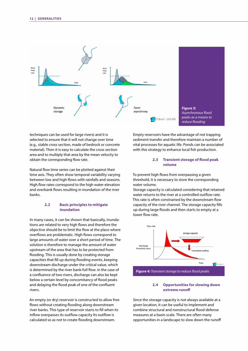
In many cases, it can be shown that basically, inunda-tions are related to very high flows and therefore the objective should be to limit the flow at the place where overflows are problematic. High flows correspond to large amounts of water over a short period of time. The solution is therefore to manage the amount of water upstream of the area that has to be protected from flooding. This is usually done by creating storage capacities that fill up during flooding events, keeping downstream discharge under the critical value, which is determined by the river bank-full flow. in the case of a confluence of two rivers, discharge can also be kept below a certain level by concomitancy of flood peaks and delaying the flood peak of one of the confluent rivers.

An empty (or dry) reservoir is constructed to allow free flows without creating flooding along downstream river banks. This type of reservoir starts to fill when its inflow overpasses its outflow capacity Its outflow is calculated so as not to create flooding downstream.

Empty reservoirs have the advantage of not trapping sediment transfer and therefore maintain a number of vital processes for aquatic life. Ponds can be associated with this strategy to enhance local fish production.

2.3 Transient storage of flood peak volume

To prevent high flows from overpassing a given threshold, it is necessary to store the corresponding water volume.Storage capacity is calculated considering that retained water returns to the river at a controlled outflow rate. This rate is often constrained by the downstream flow capacity of the river channel. The storage capacity fills up during large floods and then starts to empty at a lower flow rate.

Figure 3: Asynchronous flood peaks as a means to reduce flooding

Figure 4: Transient storage to reduce flood peaks

2.4 Opportunities for slowing down extreme runoff

Since the storage capacity is not always available at a given location, it can be useful to implement and combine structural and nonstructural flood defense measures at a basin scale. There are often many opportunities in a landscape to slow down the runoff

GENERALITIES | 13

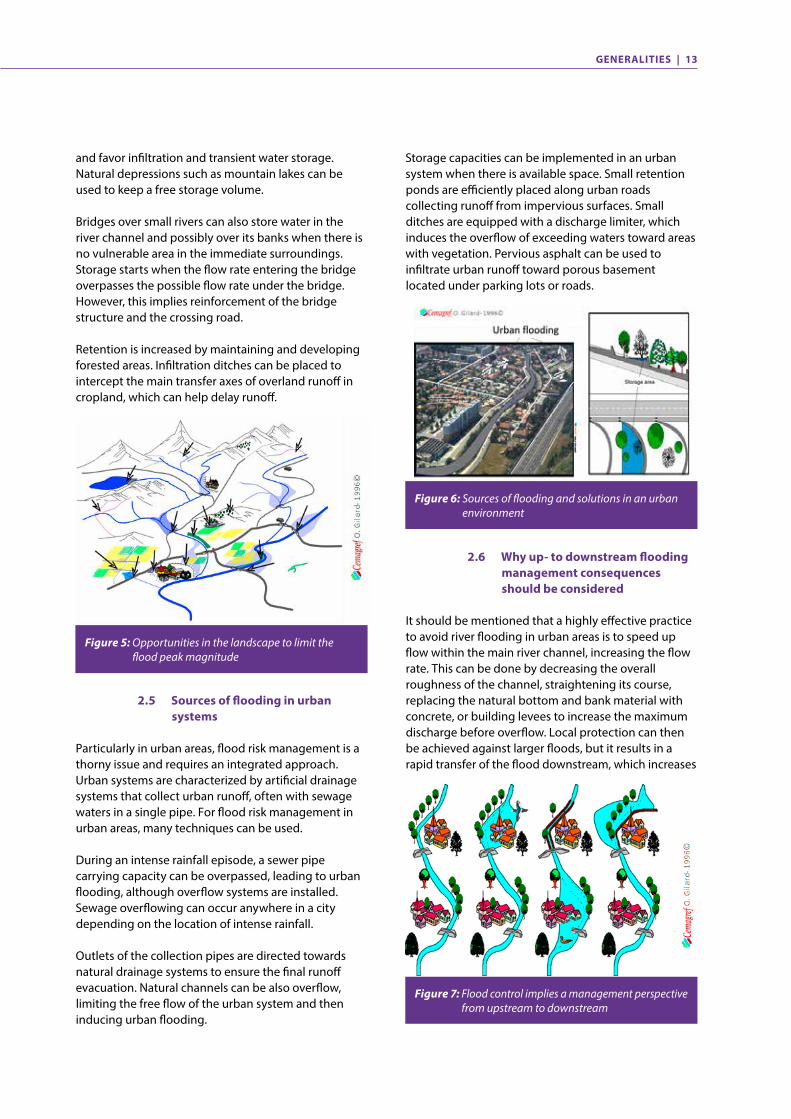
Storage capacities can be implemented in an urban system when there is available space. Small retention ponds are efficiently placed along urban roads collecting runoff from impervious surfaces. Small ditches are equipped with a discharge limiter, which induces the overflow of exceeding waters toward areas with vegetation. Pervious asphalt can be used to infiltrate urban runoff toward porous basement located under parking lots or roads.

and favor infiltration and transient water storage. Natural depressions such as mountain lakes can be used to keep a free storage volume.

Bridges over small rivers can also store water in the river channel and possibly over its banks when there is no vulnerable area in the immediate surroundings. Storage starts when the flow rate entering the bridge overpasses the possible flow rate under the bridge. However, this implies reinforcement of the bridge structure and the crossing road.

Retention is increased by maintaining and developing forested areas. Infiltration ditches can be placed to intercept the main transfer axes of overland runoff in cropland, which can help delay runoff.

2.6 Why up- to downstream flooding management consequences should be considered

It should be mentioned that a highly effective practice to avoid river flooding in urban areas is to speed up flow within the main river channel, increasing the flow rate. This can be done by decreasing the overall roughness of the channel, straightening its course, replacing the natural bottom and bank material with concrete, or building levees to increase the maximum discharge before overflow. Local protection can then be achieved against larger floods, but it results in a rapid transfer of the flood downstream, which increases

Figure 5: Opportunities in the landscape to limit the flood peak magnitude

Figure 6: Sources of flooding and solutions in an urban environment

Figure 7: Flood control implies a management perspective from upstream to downstream

2.5 Sources of flooding in urban systems

Particularly in urban areas, flood risk management is a thorny issue and requires an integrated approach.Urban systems are characterized by artificial drainage systems that collect urban runoff, often with sewage waters in a single pipe. For flood risk management in urban areas, many techniques can be used.

During an intense rainfall episode, a sewer pipe carrying capacity can be overpassed, leading to urban flooding, although overflow systems are installed. Sewage overflowing can occur anywhere in a city depending on the location of intense rainfall.

Outlets of the collection pipes are directed towards natural drainage systems to ensure the final runoff evacuation. Natural channels can be also overflow, limiting the free flow of the urban system and then inducing urban flooding.

14 | GENERALITIES

the flood hazard for downstream vulnerable areas. A more effective and a more sustainable strategy is to manage flood water volume locally and to avoid creation of new flood risk situations for downstream areas.

2.7 The effect of urbanization on flood frequency

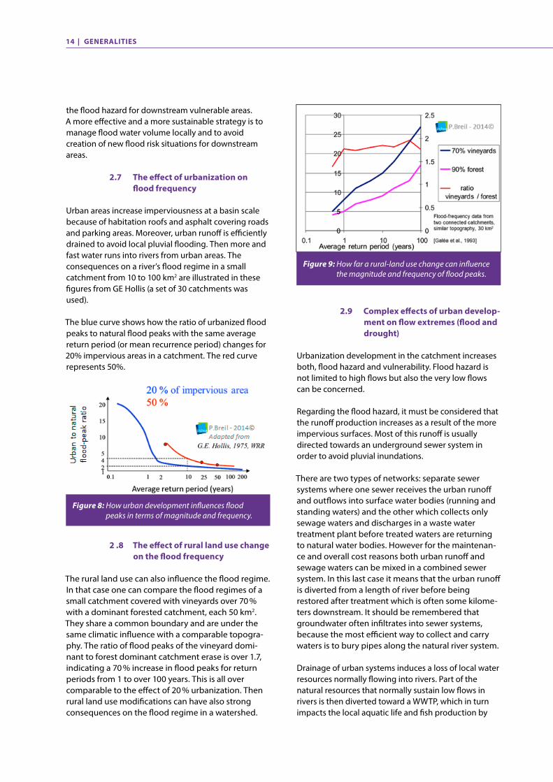
Urban areas increase imperviousness at a basin scale because of habitation roofs and asphalt covering roads and parking areas. Moreover, urban runoff is efficiently drained to avoid local pluvial flooding. Then more and fast water runs into rivers from urban areas. The consequences on a river’s flood regime in a small catchment from 10 to 100 km2 are illustrated in these figures from GE Hollis (a set of 30 catchments was used).

The blue curve shows how the ratio of urbanized flood peaks to natural flood peaks with the same average return period (or mean recurrence period) changes for 20% impervious areas in a catchment. The red curve represents 50%.

Figure 8: How urban development influences flood peaks in terms of magnitude and frequency.

Figure 9: How far a rural-land use change can influence the magnitude and frequency of flood peaks.

2 .8 The effect of rural land use change on the flood frequency

The rural land use can also influence the flood regime. In that case one can compare the flood regimes of a small catchment covered with vineyards over 70 % with a dominant forested catchment, each 50 km2. They share a common boundary and are under the same climatic influence with a comparable topogra-phy. The ratio of flood peaks of the vineyard domi-nant to forest dominant catchment erase is over 1.7, indicating a 70 % increase in flood peaks for return periods from 1 to over 100 years. This is all over comparable to the effect of 20 % urbanization. Then rural land use modifications can have also strong consequences on the flood regime in a watershed.

2.9 Complex effects of urban develop-ment on flow extremes (flood and drought)

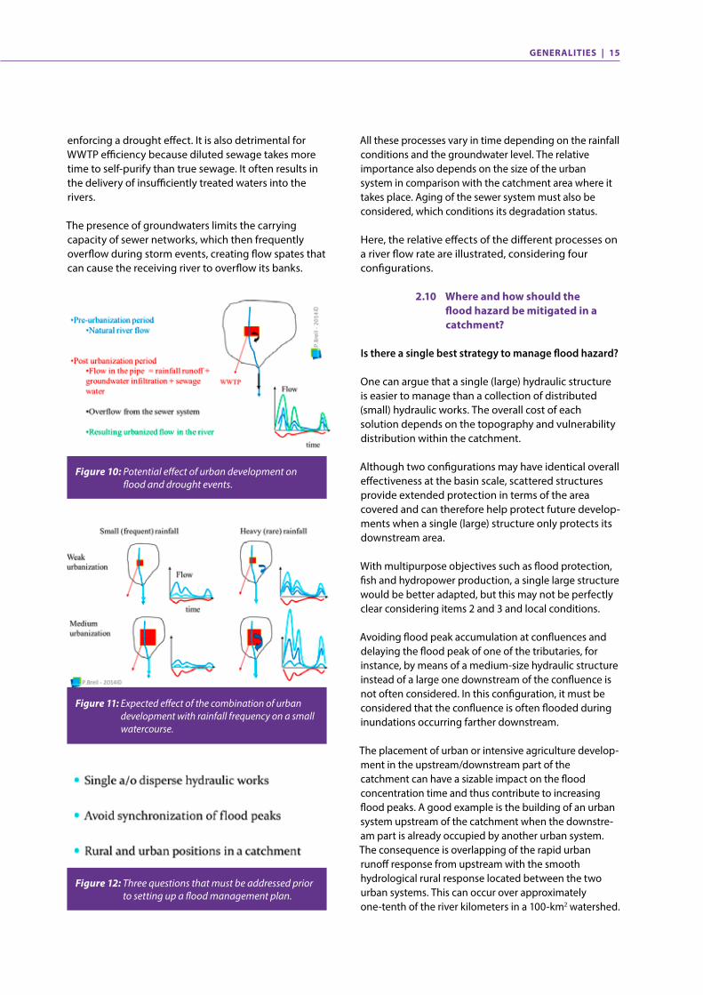
Urbanization development in the catchment increases both, flood hazard and vulnerability. Flood hazard is not limited to high flows but also the very low flows can be concerned.

Regarding the flood hazard, it must be considered that the runoff production increases as a result of the more impervious surfaces. Most of this runoff is usually directed towards an underground sewer system in order to avoid pluvial inundations.

There are two types of networks: separate sewer systems where one sewer receives the urban runoff and outflows into surface water bodies (running and standing waters) and the other which collects only sewage waters and discharges in a waste water treatment plant before treated waters are returning to natural water bodies. However for the maintenan-ce and overall cost reasons both urban runoff and sewage waters can be mixed in a combined sewer system. In this last case it means that the urban runoff is diverted from a length of river before being restored after treatment which is often some kilome-ters downstream. It should be remembered that groundwater often infiltrates into sewer systems, because the most efficient way to collect and carry waters is to bury pipes along the natural river system.

Drainage of urban systems induces a loss of local water resources normally flowing into rivers. Part of the natural resources that normally sustain low flows in rivers is then diverted toward a WWTP, which in turn impacts the local aquatic life and fish production by

GENERALITIES | 15

enforcing a drought effect. It is also detrimental for WWTP efficiency because diluted sewage takes more time to self-purify than true sewage. It often results in the delivery of insufficiently treated waters into the rivers.

The presence of groundwaters limits the carrying capacity of sewer networks, which then frequently overflow during storm events, creating flow spates that can cause the receiving river to overflow its banks.

Figure 10: Potential effect of urban development on flood and drought events.

Figure 12: Three questions that must be addressed prior to setting up a flood management plan.

Figure 11: Expected effect of the combination of urban development with rainfall frequency on a small watercourse.

All these processes vary in time depending on the rainfall conditions and the groundwater level. The relative importance also depends on the size of the urban system in comparison with the catchment area where it takes place. Aging of the sewer system must also be considered, which conditions its degradation status.

Here, the relative effects of the different processes on a river flow rate are illustrated, considering four configurations.

2.10 Where and how should the flood hazard be mitigated in a catchment?

Is there a single best strategy to manage flood hazard?

One can argue that a single (large) hydraulic structure is easier to manage than a collection of distributed (small) hydraulic works. The overall cost of each solution depends on the topography and vulnerability distribution within the catchment.

Although two configurations may have identical overall effectiveness at the basin scale, scattered structures provide extended protection in terms of the area covered and can therefore help protect future develop-ments when a single (large) structure only protects its downstream area.

With multipurpose objectives such as flood protection, fish and hydropower production, a single large structure would be better adapted, but this may not be perfectly clear considering items 2 and 3 and local conditions.

Avoiding flood peak accumulation at confluences and delaying the flood peak of one of the tributaries, for instance, by means of a medium-size hydraulic structure instead of a large one downstream of the confluence is not often considered. In this configuration, it must be considered that the confluence is often flooded during inundations occurring farther downstream.

The placement of urban or intensive agriculture develop-ment in the upstream/downstream part of the catchment can have a sizable impact on the flood concentration time and thus contribute to increasing flood peaks. A good example is the building of an urban system upstream of the catchment when the downstre-am part is already occupied by another urban system. The consequence is overlapping of the rapid urban runoff response from upstream with the smooth hydrological rural response located between the two urban systems. This can occur over approximately one-tenth of the river kilometers in a 100-km2 watershed.

16 | GENERALITIES

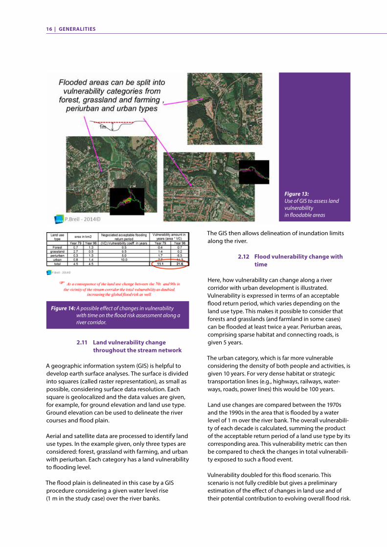
The GIS then allows delineation of inundation limits along the river.

2.12 Flood vulnerability change with time

Here, how vulnerability can change along a river corridor with urban development is illustrated. Vulnerability is expressed in terms of an acceptable flood return period, which varies depending on the land use type. This makes it possible to consider that forests and grasslands (and farmland in some cases) can be flooded at least twice a year. Periurban areas, comprising sparse habitat and connecting roads, is given 5 years.

The urban category, which is far more vulnerable considering the density of both people and activities, is given 10 years. For very dense habitat or strategic transportation lines (e.g., highways, railways, water-ways, roads, power lines) this would be 100 years.

Land use changes are compared between the 1970s and the 1990s in the area that is flooded by a water level of 1 m over the river bank. The overall vulnerabili-ty of each decade is calculated, summing the product of the acceptable return period of a land use type by its corresponding area. This vulnerability metric can then be compared to check the changes in total vulnerabili-ty exposed to such a flood event.

Vulnerability doubled for this flood scenario. This scenario is not fully credible but gives a preliminary estimation of the effect of changes in land use and of their potential contribution to evolving overall flood risk.

Figure 13: Use of GIS to assess land vulnerability in floodable areas

Figure 14: A possible effect of changes in vulnerability with time on the flood risk assessment along a river corridor.

2.11 Land vulnerability change throughout the stream network

A geographic information system (GIS) is helpful to develop earth surface analyses. The surface is divided into squares (called raster representation), as small as possible, considering surface data resolution. Each square is geolocalized and the data values are given, for example, for ground elevation and land use type. Ground elevation can be used to delineate the river courses and flood plain.

Aerial and satellite data are processed to identify land use types. In the example given, only three types are considered: forest, grassland with farming, and urban with periurban. Each category has a land vulnerability to flooding level.

The flood plain is delineated in this case by a GIS procedure considering a given water level rise (1 m in the study case) over the river banks.

Considering the high-flow distribution over an indicati-ve threshold for overbank flows, there is no periodic time pattern regarding the number and intensity of flood peaks. Consequently, the flood peak distribution is not predictable over time: this is a random process. Flood peaks can be described in relation to their probability of occurrence (frequency) or recurrence

3 Flood Hazard Modeling

3.1 Flow and flood predictability

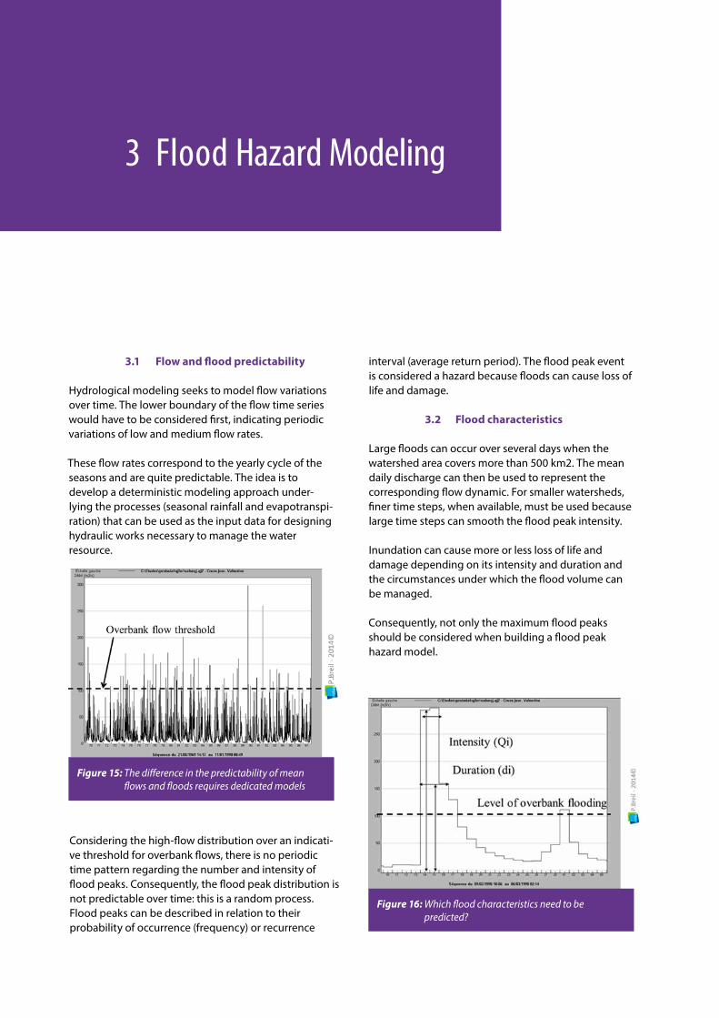
Hydrological modeling seeks to model flow variations over time. The lower boundary of the flow time series would have to be considered first, indicating periodic variations of low and medium flow rates.

These flow rates correspond to the yearly cycle of the seasons and are quite predictable. The idea is to develop a deterministic modeling approach under-lying the processes (seasonal rainfall and evapotranspi-ration) that can be used as the input data for designing hydraulic works necessary to manage the water resource.

interval (average return period). The flood peak event is considered a hazard because floods can cause loss of life and damage.

3.2 Flood characteristics

Large floods can occur over several days when the watershed area covers more than 500 km2. The mean daily discharge can then be used to represent the corresponding flow dynamic. For smaller watersheds, finer time steps, when available, must be used because large time steps can smooth the flood peak intensity.

Inundation can cause more or less loss of life and damage depending on its intensity and duration and the circumstances under which the flood volume can be managed.

Consequently, not only the maximum flood peaks should be considered when building a flood peak hazard model.

Figure 15: The difference in the predictability of mean flows and floods requires dedicated models

Figure 16: Which flood characteristics need to be predicted?

18 | FLOOD HAZARD MODELING

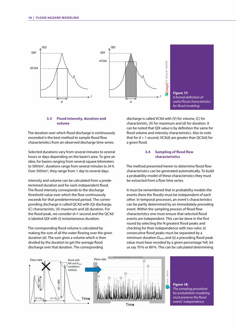
3.3 Flood intensity, duration and volume

The duration over which flood discharge is continuously exceeded is the best method to sample flood flow characteristics from an observed discharge time series.

Selected durations vary from several minutes to several hours or days depending on the basin’s area. To give an idea, for basins ranging from several square kilometers to 500 km2, durations range from several minutes to 24 h. Over 500 km2, they range from 1 day to several days.

Intensity and volume can be calculated from a prede-termined duration and for each independent flood. The flood intensity corresponds to the discharge threshold value over which the flow continuously exceeds for that predetermined period. The corres-ponding discharge is called QCXd with (Q) discharge, (C) characteristic, (X) maximum and (d) duration. For the flood peak, we consider d=1 second and the QCXd is labeled QIX with (I) instantaneous duration.

The corresponding flood volume is calculated by making the sum of all the water flowing over the given duration (d). The sum gives a volume which is then divided by the duration to get the average flood discharge over that duration. The corresponding

discharge is called VCXd with (V) for volume, (C) for characteristic, (X) for maximum and (d) for duration. It can be noted that QIX value is by definition the same for flood volume and intensity characteristics. Also to note that for d > 1 second, VCX(d) are greater than QCX(d) for a given flood.

3.4 Sampling of flood flow characteristics

The method presented herein to determine flood flow characteristics can be generated automatically. To build a probability model of these characteristics they must be extracted from a flow time series.

It must be remembered that in probability models the events (here the floods) must be independent of each other. In temporal processes, an event’s characteristics can be partly determined by an immediately preceding event. Within the sampling process of flood flow characteristics one must ensure that selected flood events are independent. This can be done in the first round by selecting the N greatest flood peaks and checking for their independence with two rules: (i) consecutive flood peaks must be separated by a minimum duration Dmin and (ii) a preceding flood peak value must have receded by a given percentage %R, let us say 70 % or 80 %. This can be calculated determining

Figure 18: The sampling procedure for probabilistic modeling must preserve the flood events’ independence.

Figure 17: A formal definition of useful flood characteristics for flood modeling

FLOOD HAZARD MODELING | 19

Figure 19: How does the sampling procedure for QCXd work on a flow time series?

Figure 20: How does the sampling procedure for VCXd work on a flow time series?

number of flood events as the number of years N in the time series. To simulate the 0.5-year flood (which occurs on average twice a year), 2 × N years must be sampled. There is however a limit because it is not possible to sample frequent (ie small) floods because their independence cannot be achieved.

3.5 QCXd sampling process

The following is an illustration of how the sampling of flood characteristics is processed by the computer. After the requested number of floods have been selected, it is necessary to check that the flood events are independent. Here the second flood is rejected due to its dependence on the first; the QCXs corres-ponding to the flood peaks are labeled QIX. They are determined using the shorter duration during which no peak discharge variation can be denoted. For large watersheds it is 1 day and for small watershed it ranges from 1 second to several hours.. The same process is performed for QCX(d) with durations greater than the minimum value d.

3.6 VCXd sampling process

The same process is used to calculate VCXd values. One can deduce from the definition of QCX and VCX that the QIX values remain the same.

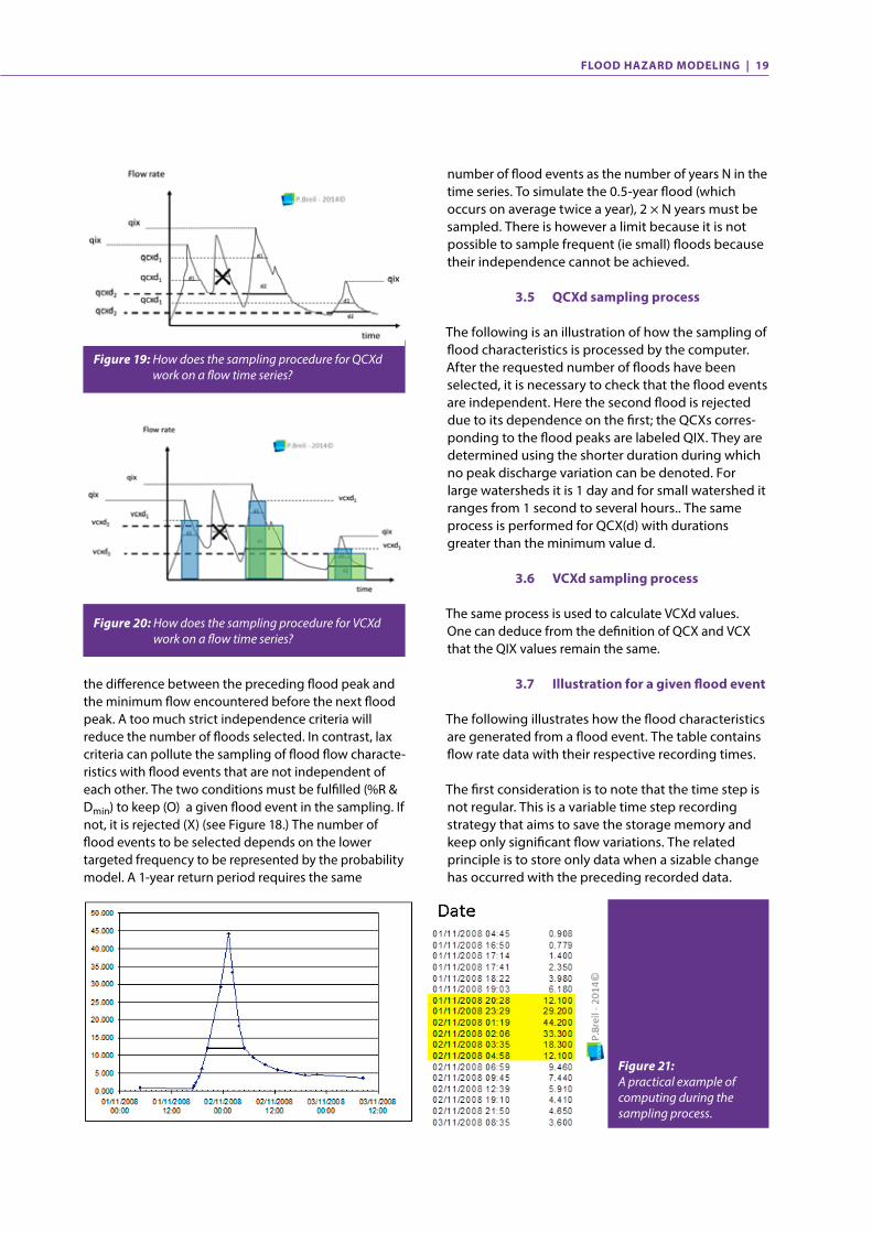
3.7 Illustration for a given flood event

The following illustrates how the flood characteristics are generated from a flood event. The table contains flow rate data with their respective recording times.

The first consideration is to note that the time step is not regular. This is a variable time step recording strategy that aims to save the storage memory and keep only significant flow variations. The related principle is to store only data when a sizable change has occurred with the preceding recorded data.

Figure 21: A practical example of computing during the sampling process.

the difference between the preceding flood peak and the minimum flow encountered before the next flood peak. A too much strict independence criteria will reduce the number of floods selected. In contrast, lax criteria can pollute the sampling of flood flow characte-ristics with flood events that are not independent of each other. The two conditions must be fulfilled (%R & Dmin) to keep (O) a given flood event in the sampling. If not, it is rejected (X) (see Figure 18.) The number of flood events to be selected depends on the lower targeted frequency to be represented by the probability model. A 1-year return period requires the same


Using data given in Figure 21. • What is the QIX value of this flood event? • What is the duration d of the yellow zone in

hourly units? • What is the value of QCX for this duration? • What is the value of VCX for this duration? How

can its calculation be implemented?

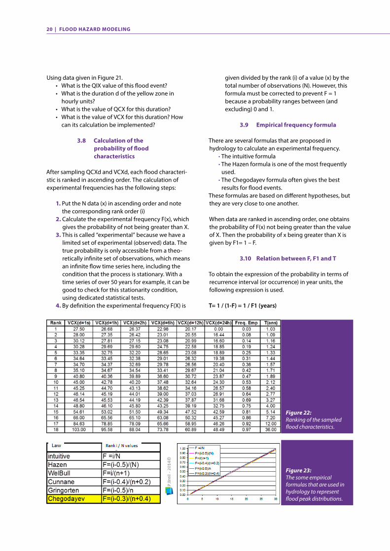
3.8 Calculation of the probability of flood characteristics

After sampling QCXd and VCXd, each flood characteri-stic is ranked in ascending order. The calculation of experimental frequencies has the following steps:

1. Put the N data (x) in ascending order and note the corresponding rank order (i)

2. Calculate the experimental frequency F(x), which gives the probability of not being greater than X.

3. This is called “experimental” because we have a limited set of experimental (observed) data. The true probability is only accessible from a theo-retically infinite set of observations, which means an infinite flow time series here, including the condition that the process is stationary. With a time series of over 50 years for example, it can be good to check for this stationarity condition, using dedicated statistical tests.

4. By definition the experimental frequency F(X) is

Figure 22: Ranking of the sampled flood characteristics.

Figure 23: The some empirical formulas that are used in hydrology to represent flood peak distributions.

given divided by the rank (i) of a value (x) by the total number of observations (N). However, this formula must be corrected to prevent F = 1 because a probability ranges between (and excluding) 0 and 1.

3.9 Empirical frequency formula

There are several formulas that are proposed in hydrology to calculate an experimental frequency. · The intuitive formula · The Hazen formula is one of the most frequently

used. · The Chegodayev formula often gives the best

results for flood events. These formulas are based on different hypotheses, but they are very close to one another. When data are ranked in ascending order, one obtains the probability of F(x) not being greater than the value of X. Then the probability of x being greater than X is given by F1= 1 – F.

3.10 Relation between F, F1 and T

To obtain the expression of the probability in terms of recurrence interval (or occurrence) in year units, the following expression is used.

T= 1 / (1-F) = 1 / F1 (years)


This has the advantage of making the probability more obvious to decision-makers. However, it should be remembered that over a 100-year period there are on average ten flood events near the 10-year return period flood that can occur randomly rather than syste-matically every 10 years.

A random value associated with its probability of being greater (or lesser) than this value is called a quantile, which represents a partition of the probability density function of this variable.

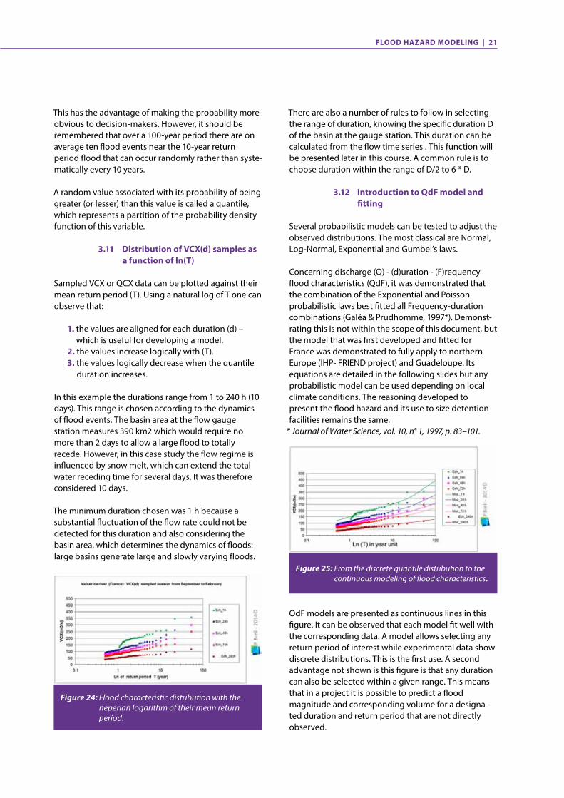
3.11 Distribution of VCX(d) samples as a function of ln(T)

Sampled VCX or QCX data can be plotted against their mean return period (T). Using a natural log of T one can observe that:

1. the values are aligned for each duration (d) – which is useful for developing a model.

2. the values increase logically with (T). 3. the values logically decrease when the quantile

duration increases.

In this example the durations range from 1 to 240 h (10 days). This range is chosen according to the dynamics of flood events. The basin area at the flow gauge station measures 390 km2 which would require no more than 2 days to allow a large flood to totally recede. However, in this case study the flow regime is influenced by snow melt, which can extend the total water receding time for several days. It was therefore considered 10 days.

The minimum duration chosen was 1 h because a substantial fluctuation of the flow rate could not be detected for this duration and also considering the basin area, which determines the dynamics of floods: large basins generate large and slowly varying floods.

There are also a number of rules to follow in selecting the range of duration, knowing the specific duration D of the basin at the gauge station. This duration can be calculated from the flow time series . This function will be presented later in this course. A common rule is to choose duration within the range of D/2 to 6 * D.

3.12 Introduction to QdF model and fitting

Several probabilistic models can be tested to adjust the observed distributions. The most classical are Normal, Log-Normal, Exponential and Gumbel’s laws.

Concerning discharge (Q) - (d)uration - (F)requency flood characteristics (QdF), it was demonstrated that the combination of the Exponential and Poisson probabilistic laws best fitted all Frequency-duration combinations (Galéa & Prudhomme, 1997*). Demonst-rating this is not within the scope of this document, but the model that was first developed and fitted for France was demonstrated to fully apply to northern Europe (IHP- FRIEND project) and Guadeloupe. Its equations are detailed in the following slides but any probabilistic model can be used depending on local climate conditions. The reasoning developed to present the flood hazard and its use to size detention facilities remains the same.

* Journal of Water Science, vol. 10, n° 1, 1997, p. 83–101.

Figure 24: Flood characteristic distribution with the neperian logarithm of their mean return period.

OdF models are presented as continuous lines in this figure. It can be observed that each model fit well with the corresponding data. A model allows selecting any return period of interest while experimental data show discrete distributions. This is the first use. A second advantage not shown is this figure is that any duration can also be selected within a given range. This means that in a project it is possible to predict a flood magnitude and corresponding volume for a designa-ted duration and return period that are not directly observed.

Figure 25: From the discrete quantile distribution to the continuous modeling of flood characteristics.


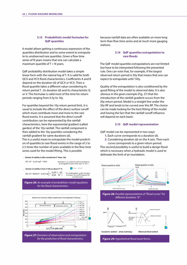
3.13 Probabilistic model formulae for QdF quantiles

A model allows getting a continuous expression of the quantiles distribution and to some extent to extrapola-te to unobserved rare quantiles. Given a flow time series of N years means that one can calculate a maximum quantile of T = N years.

QdF probability distribution model takes a simple linear form with the natural log of T. It is valid for both QCX and VCX flood characteristics. Coefficients A and B depend on the duration (d) of QCX or VCX. Then a flood quantile takes a different value considering its return period T , its duration (d) and its characteristic Q or V. This formulae is valid most of the time for return periods ranging from 0.5y to 10y.

For quantiles beyond the 10y return period limit, it is usual to include the effect of the direct surface runoff which must contribute more and more to the rare flood events. It is assumed that the direct runoff contribution can be represented by the rainfall characteristics, here the exponential gradient (called gardex) of the 10y rainfall. The rainfall component is then added to the 10y quantiles considering the rainfall gradient for same durations (d). This is a useful mean to extrapolate the model predicti-on of quantiles to rare flood events in the range of 2 to 2.5 times the number of years available in the flow time series used for the model fitting. This is possible

Figure 26: An example of probabilistic model equations for the flood characteristics.

Figure 28: Possible representations of "flood curves” for different durations "d".

Figure 29: Hypothetical flood event forms.Figure 27: Domains of observation and extrapolation

for the prediction of flood characteristics.

because rainfall data are often available on more long term than flow time series and at much more gauging stations.

3.14 QdF quantiles extrapolation to rare floods

The QdF model quantiles extrapolations are not limited but have to be interpreted following the presented rule. One can note that, for example, if the largest observed return period is 50y that means that one can expect to extrapolate until 150y.

Quality of the extrapolation is also conditioned by the good fitting of the model to observed data. It is also obvious in the given exemple (Fig. 27) that the introduction of the rainfall gradient occurs from the 20y return period. Model is a straight line under the 20y RP and tends to be curved over this RP. The choice can be made looking for the best fitting of the model and having the fact that the rainfall runoff influence will depend on each basin.

3.15 QdF model representation

QdF model can be represented in two ways: 1. Each curve corresponds to a duration (d). 2. Considering duration (d) on the X-axis. Then each

curve corresponds to a given return period.This second possibility is useful to build a design flood which is necessary when a hydraulic model is used to delineate the limit of an inundation.


3.16 Methods for designing floods

The main limitation of these methods is that only the flood peaks are taken for the known return period. This means the inundation limit given by a hydraulic model using these designed floods would change with other flood patterns while the flood peak remains the same. The return period of the flood limit is then not known.

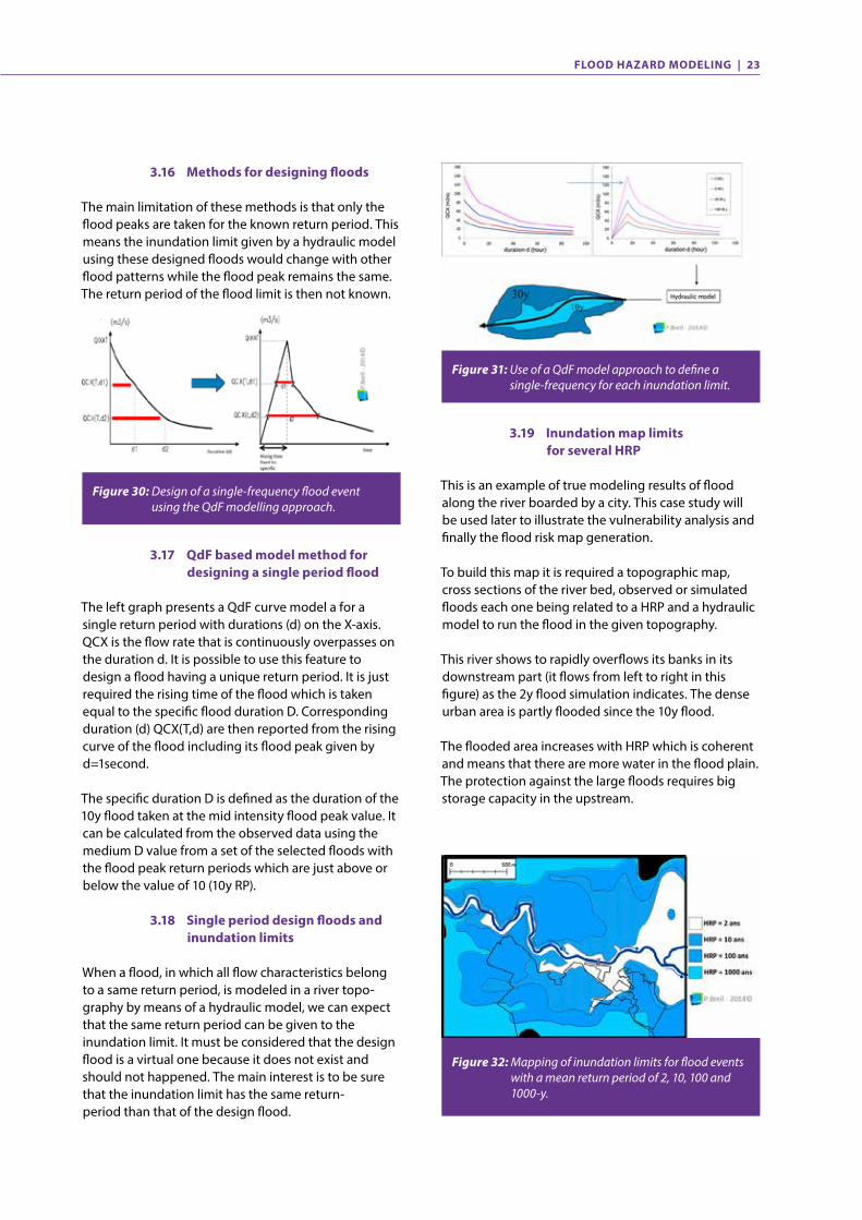
3.19 Inundation map limits for several HRP

This is an example of true modeling results of flood along the river boarded by a city. This case study will be used later to illustrate the vulnerability analysis and finally the flood risk map generation.

To build this map it is required a topographic map, cross sections of the river bed, observed or simulated floods each one being related to a HRP and a hydraulic model to run the flood in the given topography.

This river shows to rapidly overflows its banks in its downstream part (it flows from left to right in this figure) as the 2y flood simulation indicates. The dense urban area is partly flooded since the 10y flood.

The flooded area increases with HRP which is coherent and means that there are more water in the flood plain. The protection against the large floods requires big storage capacity in the upstream.

Figure 30: Design of a single-frequency flood event using the QdF modelling approach.

Figure 31: Use of a QdF model approach to define a single-frequency for each inundation limit.

Figure 32: Mapping of inundation limits for flood events with a mean return period of 2, 10, 100 and 1000-y.

3.17 QdF based model method for designing a single period flood

The left graph presents a QdF curve model a for a single return period with durations (d) on the X-axis. QCX is the flow rate that is continuously overpasses on the duration d. It is possible to use this feature to design a flood having a unique return period. It is just required the rising time of the flood which is taken equal to the specific flood duration D. Corresponding duration (d) QCX(T,d) are then reported from the rising curve of the flood including its flood peak given by d=1second.

The specific duration D is defined as the duration of the 10y flood taken at the mid intensity flood peak value. It can be calculated from the observed data using the medium D value from a set of the selected floods with the flood peak return periods which are just above or below the value of 10 (10y RP).

3.18 Single period design floods and inundation limits

When a flood, in which all flow characteristics belong to a same return period, is modeled in a river topography by means of a hydraulic model, we can expect that the same return period can be given to the inundation limit. It must be considered that the design flood is a virtual one because it does not exist and should not happened. The main interest is to be sure that the inundation limit has the same return- period than that of the design flood.


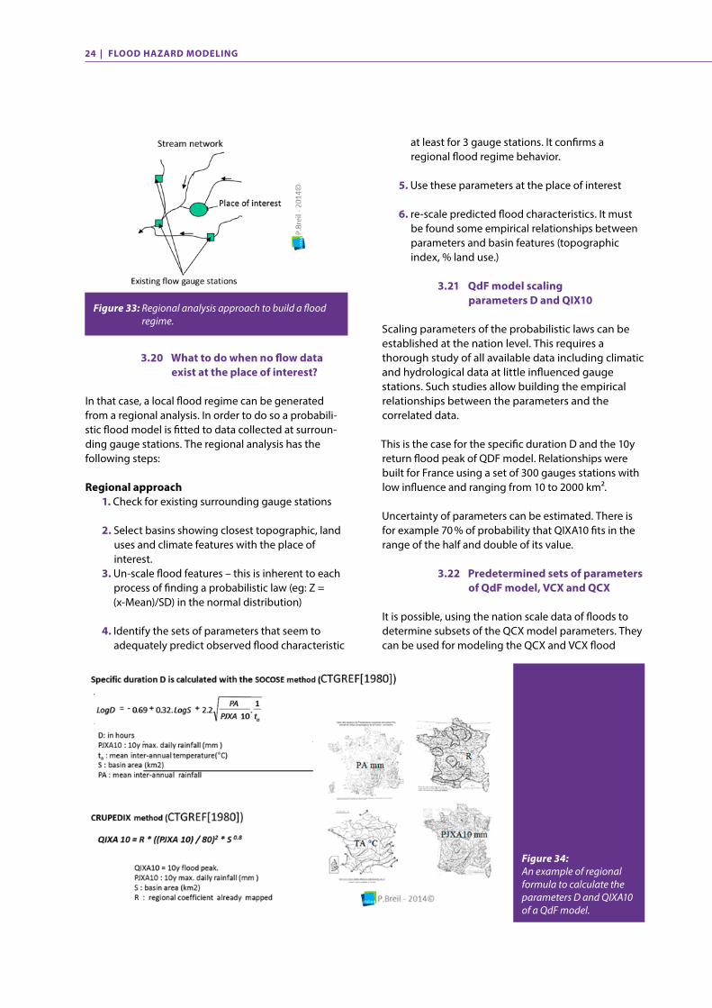
at least for 3 gauge stations. It confirms a regional flood regime behavior.

5. Use these parameters at the place of interest

6. re-scale predicted flood characteristics. It must be found some empirical relationships between parameters and basin features (topographic index, % land use.)

3.21 QdF model scaling parameters D and QIX10

Scaling parameters of the probabilistic laws can be established at the nation level. This requires a thorough study of all available data including climatic and hydrological data at little influenced gauge stations. Such studies allow building the empirical relationships between the parameters and the correlated data.

This is the case for the specific duration D and the 10y return flood peak of QDF model. Relationships were built for France using a set of 300 gauges stations with low influence and ranging from 10 to 2000 km2.

Uncertainty of parameters can be estimated. There is for example 70 % of probability that QIXA10 fits in the range of the half and double of its value.

3.22 Predetermined sets of parameters of QdF model, VCX and QCX

It is possible, using the nation scale data of floods to determine subsets of the QCX model parameters. They can be used for modeling the QCX and VCX flood

Figure 33: Regional analysis approach to build a flood regime.

3.20 What to do when no flow data exist at the place of interest?

In that case, a local flood regime can be generated from a regional analysis. In order to do so a probabili-stic flood model is fitted to data collected at surroun-ding gauge stations. The regional analysis has the following steps:

Regional approach 1. Check for existing surrounding gauge stations

2. Select basins showing closest topographic, land uses and climate features with the place of interest.

3. Un-scale flood features – this is inherent to each process of finding a probabilistic law (eg: Z = (x-Mean)/SD) in the normal distribution)

4. Identify the sets of parameters that seem to adequately predict observed flood characteristic

Figure 34: An example of regional formula to calculate the parameters D and QIXA10 of a QdF model.


Figure 36: Principle for the predetermination of a storage capacity for a flood event using a constant flow rate release.

Figure 35: Predetermined sets of parameters of QdF model, VCX and QCX.

regimes in a geographic area where no gauge station is available. This is called regional hydrology.

Values of Xi parameters can be tabulated and the Xi values can be “un-scaled” using two flood characteri-stics of basins: its 10 years flood peak (QIXA10) and its specific duration (D) which can be assimilated to its time of concentration.

The procedure to identify which set of Xi parameters best fit to QCX and VCX extracted from a gauge station is then to re-scale predicted values using these two flood characteristics which can be extracted directly from the sampled floods or using a national fitted empirical relationship which has been presented just before.

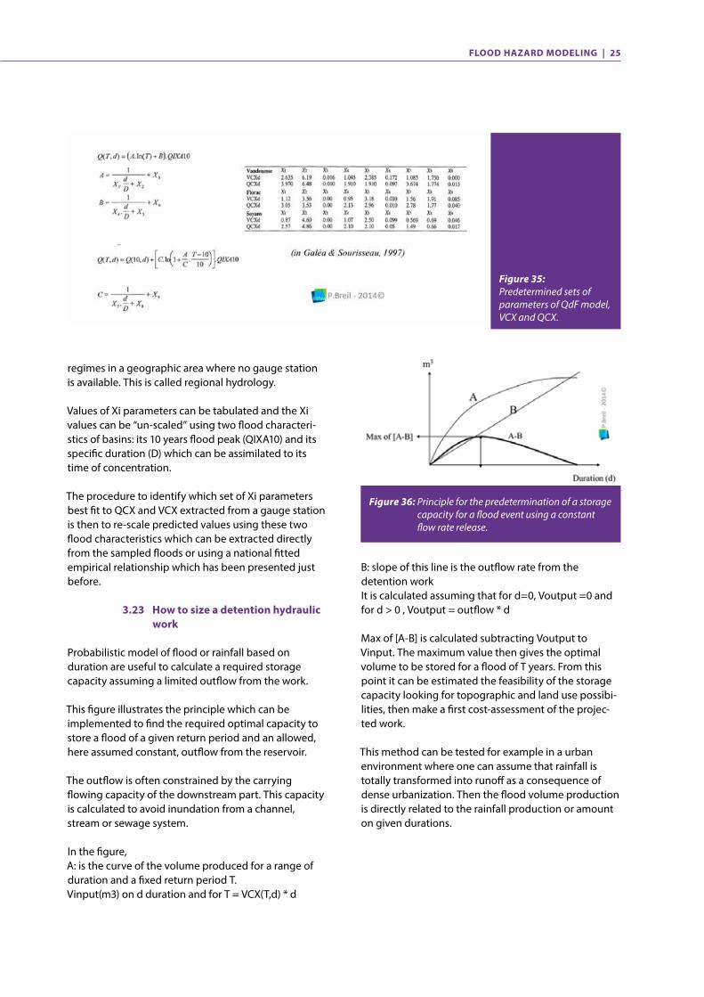
3.23 How to size a detention hydraulic work

Probabilistic model of flood or rainfall based on duration are useful to calculate a required storage capacity assuming a limited outflow from the work.

This figure illustrates the principle which can be implemented to find the required optimal capacity to store a flood of a given return period and an allowed, here assumed constant, outflow from the reservoir.

The outflow is often constrained by the carrying flowing capacity of the downstream part. This capacity is calculated to avoid inundation from a channel, stream or sewage system.

In the figure, A: is the curve of the volume produced for a range of duration and a fixed return period T. Vinput(m3) on d duration and for T = VCX(T,d) * d

B: slope of this line is the outflow rate from the detention workIt is calculated assuming that for d=0, Voutput =0 and for d > 0 , Voutput = outflow * d

Max of [A-B] is calculated subtracting Voutput to Vinput. The maximum value then gives the optimal volume to be stored for a flood of T years. From this point it can be estimated the feasibility of the storage capacity looking for topographic and land use possibi-lities, then make a first cost-assessment of the projec-ted work.

This method can be tested for example in a urban environment where one can assume that rainfall is totally transformed into runoff as a consequence of dense urbanization. Then the flood volume production is directly related to the rainfall production or amount on given durations.

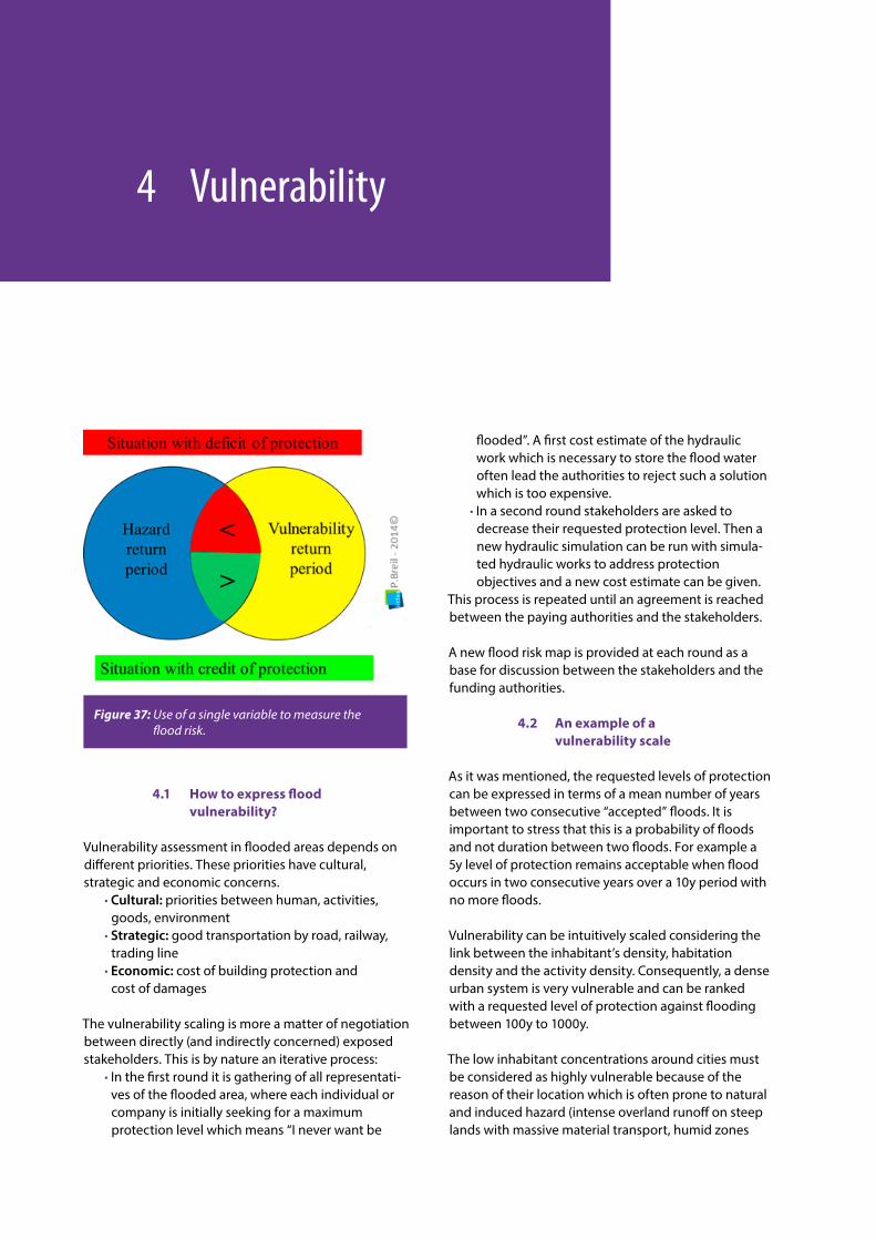
4.1 How to express flood vulnerability?

Vulnerability assessment in flooded areas depends on different priorities. These priorities have cultural, strategic and economic concerns. · Cultural: priorities between human, activities,

goods, environment · Strategic: good transportation by road, railway,

trading line · Economic: cost of building protection and

cost of damages

The vulnerability scaling is more a matter of negotiation between directly (and indirectly concerned) exposed stakeholders. This is by nature an iterative process: · In the first round it is gathering of all representati-

ves of the flooded area, where each individual or company is initially seeking for a maximum protection level which means “I never want be

4 Vulnerability

4.1 How to express flood vulnerability?

flooded”. A first cost estimate of the hydraulic work which is necessary to store the flood water often lead the authorities to reject such a solution which is too expensive.

· In a second round stakeholders are asked to decrease their requested protection level. Then a new hydraulic simulation can be run with simula-ted hydraulic works to address protection objectives and a new cost estimate can be given.

This process is repeated until an agreement is reached between the paying authorities and the stakeholders.

A new flood risk map is provided at each round as a base for discussion between the stakeholders and the funding authorities.

4.2 An example of a vulnerability scale

As it was mentioned, the requested levels of protection can be expressed in terms of a mean number of years between two consecutive “accepted” floods. It is important to stress that this is a probability of floods and not duration between two floods. For example a 5y level of protection remains acceptable when flood occurs in two consecutive years over a 10y period with no more floods.

Vulnerability can be intuitively scaled considering the link between the inhabitant’s density, habitation density and the activity density. Consequently, a dense urban system is very vulnerable and can be ranked with a requested level of protection against flooding between 100y to 1000y.

The low inhabitant concentrations around cities must be considered as highly vulnerable because of the reason of their location which is often prone to natural and induced hazard (intense overland runoff on steep lands with massive material transport, humid zones

Figure 37: Use of a single variable to measure the flood risk.

28 | VULNERABILITY

prone to inundation, low capacity to rebuild, lack of information during flood event and sanitary problems after events). In this case vulnerability is mainly human inhabitants concerned and should be rate at least 100y. To disperse habitat is always given the lower vulnerabi-lity rates. That is also because of the possibilities for people to move away and secure their goods in an easier way than in the dense urban areas.

Also, the communication networks are very sensitive and transportation ways, in particular because they convey people and goods. Any long service disruption has consequences on the locals and sometimes for the economy. Short interruptions can endanger people because of lack of awareness given by the authorities due to rapid floods. In that case it is necessary to develop information and educate people on the behavior they must have when a flash flood occurs. This is a good mean to enhance the resilience capacity of a popoulation to flooding. A rate of 100y can be given for dense traffic lines like for highways and the fast trains.

Rural lands are then less vulnerable to flood and can be rated with the lower protection levels. However, that is not true everywhere when one considers farming as a basic resource for families. Distinction must be made between the rural land uses in term of requested flood protection level.

Lands surrounded by water during flooding become isolated with no chance for people to easily escape. These are very critical situations which require adapted warning and training of residents because it is not possible to protect them.

Vulnerability can also be scaled considering the specific aspects of flood events like water depth, duration of submersion and the flow velocity. These flood charac-teristic are physically related at a given place which

means that they are not independent and fully constrained by the local topography.

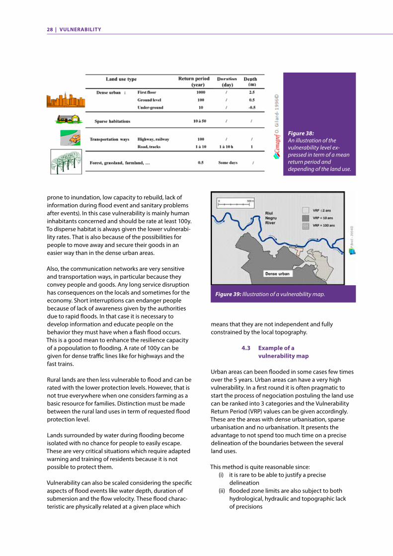
4.3 Example of a vulnerability map

Urban areas can been flooded in some cases few times over the 5 years. Urban areas can have a very high vulnerability. In a first round it is often pragmatic to start the process of negociation postuling the land use can be ranked into 3 categories and the Vulnerability Return Period (VRP) values can be given accordingly. These are the areas with dense urbanisation, sparse urbanisation and no urbanisation. It presents the advantage to not spend too much time on a precise delineation of the boundaries between the several land uses.

This method is quite reasonable since: (i) it is rare to be able to justify a precise

delineation (ii) flooded zone limits are also subject to both

hydrological, hydraulic and topographic lack of precisions

Figure 38: An illustration of the vulnerability level ex-pressed in term of a mean return period and depending of the land use.

Figure 39: Illustration of a vulnerability map.

VULNERABILITY | 29

(iii) a precise delineation can attract personal interest on the frontiers which disturb a general perception of the problem to be solved.

4.4 A Cost-Benefit approach of Vulnerability

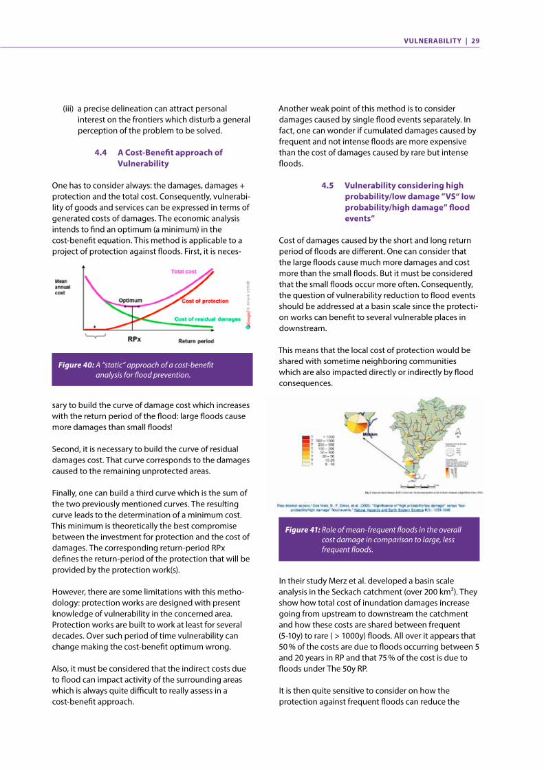
One has to consider always: the damages, damages + protection and the total cost. Consequently, vulnerabi-lity of goods and services can be expressed in terms of generated costs of damages. The economic analysis intends to find an optimum (a minimum) in the cost-benefit equation. This method is applicable to a project of protection against floods. First, it is neces-

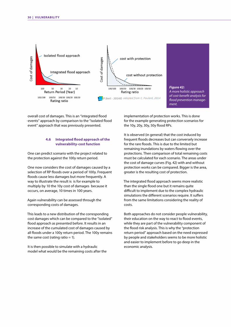
Another weak point of this method is to consider damages caused by single flood events separately. In fact, one can wonder if cumulated damages caused by frequent and not intense floods are more expensive than the cost of damages caused by rare but intense floods.

4.5 Vulnerability considering high probability/low damage ”VS“ low probability/high damage” flood events”

Cost of damages caused by the short and long return period of floods are different. One can consider that the large floods cause much more damages and cost more than the small floods. But it must be considered that the small floods occur more often. Consequently, the question of vulnerability reduction to flood events should be addressed at a basin scale since the protecti-on works can benefit to several vulnerable places in downstream.

This means that the local cost of protection would be shared with sometime neighboring communities which are also impacted directly or indirectly by flood consequences.

Figure 40: A “static” approach of a cost-benefit analysis for flood prevention.

Figure 41: Role of mean-frequent floods in the overall cost damage in comparison to large, less frequent floods.

sary to build the curve of damage cost which increases with the return period of the flood: large floods cause more damages than small floods!

Second, it is necessary to build the curve of residual damages cost. That curve corresponds to the damages caused to the remaining unprotected areas.

Finally, one can build a third curve which is the sum of the two previously mentioned curves. The resulting curve leads to the determination of a minimum cost. This minimum is theoretically the best compromise between the investment for protection and the cost of damages. The corresponding return-period RPx defines the return-period of the protection that will be provided by the protection work(s).

However, there are some limitations with this metho-dology: protection works are designed with present knowledge of vulnerability in the concerned area. Protection works are built to work at least for several decades. Over such period of time vulnerability can change making the cost-benefit optimum wrong.

Also, it must be considered that the indirect costs due to flood can impact activity of the surrounding areas which is always quite difficult to really assess in a cost-benefit approach.

In their study Merz et al. developed a basin scale analysis in the Seckach catchment (over 200 km2). They show how total cost of inundation damages increase going from upstream to downstream the catchment and how these costs are shared between frequent (5-10y) to rare ( > 1000y) floods. All over it appears that 50 % of the costs are due to floods occurring between 5 and 20 years in RP and that 75 % of the cost is due to floods under The 50y RP.

It is then quite sensitive to consider on how the protection against frequent floods can reduce the

30 | VULNERABILITY

overall cost of damages. This is an “integrated flood -events” approach by comparison to the “isolated flood event” approach that was previously presented.

4.6 Integrated flood approach of the vulnerability-cost function

One can predict scenario with the project related to the protection against the 100y return period.

One now considers the cost of damages caused by a selection of RP floods over a period of 100y. Frequent floods cause less damages but more frequently. A way to illustrate the result is is for example to multiply by 10 the 10y cost of damages because it occurs, on average, 10 times in 100 years.

Again vulnerability can be assessed through the corresponding costs of damages.

This leads to a new distribution of the corresponding cost damages which can be compared to the “isolated” flood approach as presented before. It results in an increase of the cumulated cost of damages caused by all floods under a 100y return period. The 100y remains the same cost (rating ratio = 1).

It is then possible to simulate with a hydraulic model what would be the remaining costs after the

implementation of protection works. This is done for the example generating protection scenarios for the 10y, 20y, 30y, 50y flood RPs.

It is observed (in general) that the cost induced by frequent floods decreases but can conversely increase for the rare floods. This is due to the limited but remaining inundations by waters flowing over the protections. Then comparison of total remaining costs must be calculated for each scenario. The areas under the cost of damage curves (Fig. 42) with and without protection works can be compared. Bigger is the area, greater is the resulting cost of protection.

The integrated flood approach seems more realistic than the single flood one but it remains quite difficult to implement due to the complex hydraulic simulations the different scenarios require. It suffers from the same limitations considering the reality of costs.

Both approaches do not consider people vulnerability, their education on the way to react to flood events, while they are part of the vulnerability component of the flood risk analysis. This is why the “protection return period” approach based on the need expressed by people and stakeholders seems to be more holistic and easier to implement before to go deep in theeconomic analysis.

Figure 42: A more holistic approach of cost-benefit analysis for flood prevention manage-ment.

5 Flood risk mapping

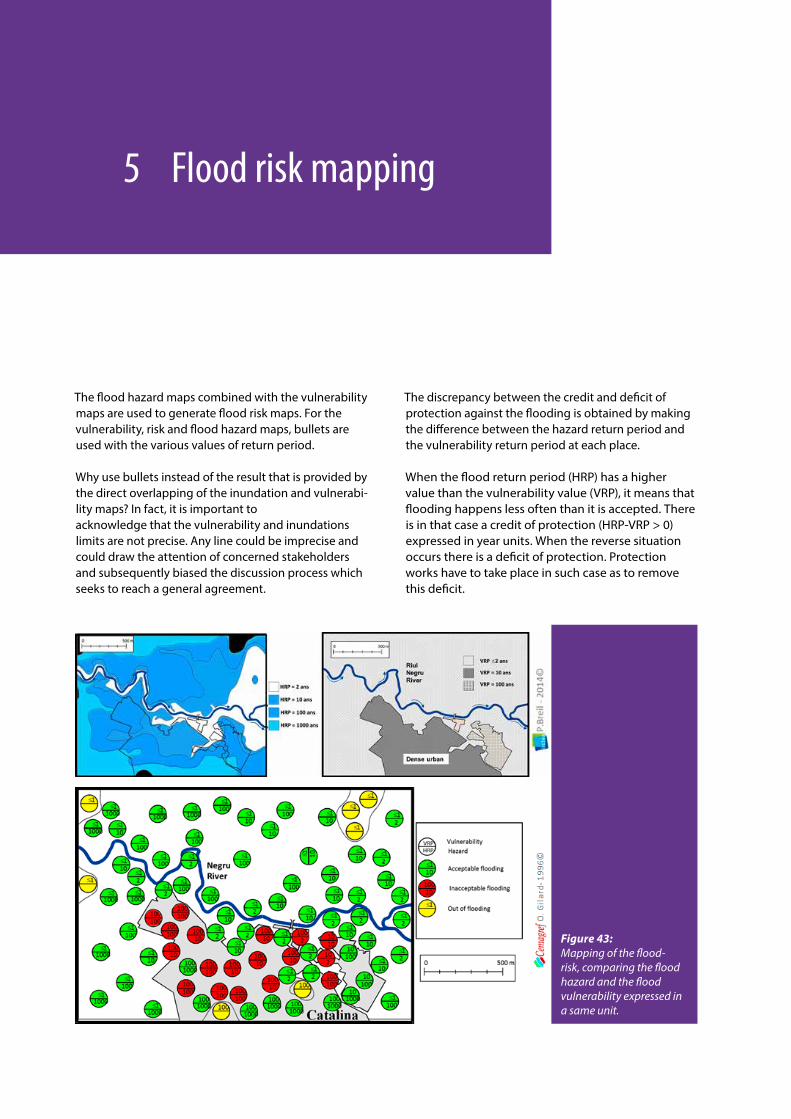
The flood hazard maps combined with the vulnerability maps are used to generate flood risk maps. For the vulnerability, risk and flood hazard maps, bullets are used with the various values of return period.

Why use bullets instead of the result that is provided by the direct overlapping of the inundation and vulnerabi-lity maps? In fact, it is important to acknowledge that the vulnerability and inundations limits are not precise. Any line could be imprecise and could draw the attention of concerned stakeholders and subsequently biased the discussion process which seeks to reach a general agreement.

Figure 43: Mapping of the flood-risk, comparing the flood hazard and the flood vulnerability expressed in a same unit.

The discrepancy between the credit and deficit of protection against the flooding is obtained by making the difference between the hazard return period and the vulnerability return period at each place.

When the flood return period (HRP) has a higher value than the vulnerability value (VRP), it means that flooding happens less often than it is accepted. There is in that case a credit of protection (HRP-VRP > 0) expressed in year units. When the reverse situation occurs there is a deficit of protection. Protection works have to take place in such case as to remove this deficit.

32 | FLOOD RISK MAPPING

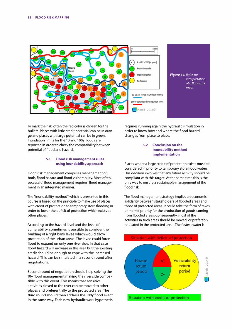
requires running again the hydraulic simulation in order to know how and where the flood hazard changes from place to place.

5.2 Conclusion on the inundability method implementation

Places where a large credit of protection exists must be considered in priority to temporary store flood waters. This decision involves that any future activity should be compliant with this target. At the same time this is the only way to ensure a sustainable management of the flood risk.

The flood management strategy implies an economic solidarity between stakeholders of flooded areas and those of protected areas. It could take the form of taxes or market priority for the production of goods coming from flooded areas. Consequently, most of the activities in such areas should be moved, or preferably relocated in the protected area. The fastest water is

Figure 44: Rules for interpretation of a flood-risk map.

To mark the risk, often the red color is chosen for the bullets. Places with little credit potential can be in oran-ge and places with large potential can be in green. Inundation limits for the 10 and 100y floods are reported in order to check the compatibility between potential of flood and hazard.

5.1 Flood risk management rules using inundability approach

Flood risk management comprises management of both, flood hazard and flood vulnerability. Most often, successful flood management requires, flood manage-ment in an integrated manner.

The “inundability method” which is presented in this course is based on the principle to make use of places with credit of protection to temporary store flooding in order to lower the deficit of protection which exists at other places.

According to the hazard level and the level of vulnerability, sometimes is possible to consider the building of a right bank levee which would allow protection of the urban areas. The levee could force flood to expand on only one river side. In that case flood hazard will increase in this area but the existing credit should be enough to cope with the increased hazard. This can be simulated in a second round after negotiations.

Second round of negotiation should help solving the 10y flood management making the river side compa-tible with this event. This means that sensitive activities closed to the river can be moved to other places and preferentially to the protected area. The third round should then address the 100y flood event in the same way. Each new hydraulic work hypothesis

FLOOD RISK MAPPING | 33

mostly issued to rivers from the urban areas. That effect has the consequences for the flood regime.

It can happen that, due to the urbanization, the 10-year return period flood is multiplied by 2. This effect is very sensitive for the floods with small return period. The urban development can increase the flood hazard and inundation process.

Rural land use change can also influence the flood regimes. That requires specific measures of flood risk

management (nature based solutions like the main-tenance of riparian corridor, forested soils on hillslopes, all practices which help to slowdown or infiltrate surface runoff before it reaches a river network). The soft protection measures can also contribute the ecosystem services protection (constructed-wetlands built at foot of hills, for trapping and creation of biomass from the fertilizers that are washed from agricultural lands). The rural land use modifications can have also strong consequences on the flood regime in a watershed which affects agriculture and the farmers.

Figure 1: A measure of the flood risk 8

Figure 2: From the hillslope runoff to the flood generation in a water course 11

Figure 3: Asynchronous flood peaks as a mean to reduce flooding. 12

Figure 4: Transient storage to reduce flood peaks. 12

Figure 5: Opportunities in the landscape to limit the flood peaks magnitude 13

Figure 6: Sources of flooding and kind of solutions in urban environment 13

Figure 7: Flood control implies a management perspective from upstream to downstream. 13

Figure 8: How the urban development influences the flood peaks in terms of magnitude and frequency. 14

Figure 9: How far a rural-land use change can influence the magnitude and frequency of flood peaks. 14

Figure 10: Potential urban development effect on flood and drought events. 15

Figure 11: Expected effect of the combination of urban development with rainfall frequency on a small water course. 15

Figure 12: Three questions that must be addressed prior the setting of a flood management plan. 15

Figure 13: Use of GIS to assess the land vulnerability in the floodable areas. 16

Figure 14: A possible effect of the vulnerability change with time on the flood risk assessment along a river corridor. 16

Figure 15: The difference in the predicatability of mean flows and floods leads to a need for dedicated models. 17

Figure 16: Which flood characteristics do we need to predict? 17

Figure 17: A formal definition of interesting flood characteristics for a modeling objective. 18

Figure 18: The sampling procedure for probabilistic modeling must preserve the flood events independency. 18

Figure 19: How does the sampling procedure for QCXd work on a flow time series? 19

Figure 20: How does the sampling procedure for VCXd work on a flow time series? 19

Figure 21: A practical example of what the computer must do during the sampling process. 19

Figure 22: Ranking of the sampled flood characteristics. 20

Figure 23: Calculation of the flood empirical frequency. 20

Figure 24: Flood characteristic distribution with the neperian logarithm of their mean return period. 21

List of Figures

36 | LIST OF FIGURES

Figure 25: From the discrete quantiles distribution to the continuous modeling of flood characteristics. 21

Figure 26: An example of probabilistic model equations for the flood characteristics. 22

Figure 27: Domains of observation and extrapolation for the prediction of flood characteristics. 22

Figure 28: Possible representations of “flood curves” for different durations ‘d’. 22

Figure 29: Hypothetical flood event forms. 22

Figure 30: Design of a single-frequency flood event using the QdF modelling approach. 23

Figure 31: Use of a QdF model approach to define a single-frequency for each inundation limit. 23

Figure 32: Mapping of inundation limits for flood events with a mean return period of 2, 10, 100 and 1000-y. 23

Figure 33: Regional analysis approach to build a flood regime. 24

Figure 34: An example of regional formula to calculate the parameters D and QIXA10 of a QdF model. 24

Figure 35: Predetermined sets of parameters of QdF model, VCX and QCX. 25

Figure 36: Principle for the predetermination of a storage capacity for a flood event using a constant flow rate release. 25

Figure 37: Use of a single variable to measure the flood risk. 27

Figure 38: An illustration of the vulnerability level expressed in term of a mean return period and depending of the land use. 28

Figure 39: Illustration of a vulnerability map. 28

Figure 40: A “static” approach of a cost-benefit analysis for flood prevention. 29

Figure 41: Role of mean-frequent floods in the overall cost damage in comparison to large, less frequent floods. 29

Figure 42: A more holistic approach of cost-benefit analysis for flood prevention management. 30

Figure 43: Mapping of the flood-risk, comparing the flood hazard and the flood vulnerability expressed in a same unit. 31

Figure 44: Rules for interpretation of a flood-risk map. 32

UNESCO Office, JakartaJl. Galuh II No. 5Kebayoran BaruJakarta 12110 • IndonesiaTelephone: +62 (21) 739 9818Telefax: +62 (21) 7279 [email protected] • www.unesco.org/jakarta

International Centre for Water Resources and Global Change Federal Institute of Hydrology • P.O. Box 20025356002 Koblenz • GermanyTelephone: +49 (0)261/1306 - 5313 Telefax: +49 (0)261/1306 - [email protected] • www.waterandchange.org








training course on flood risk assessment - icwrgc

Documents