regresi 1. 2 regresi adalah diberikan sejumlah n buah data yg dimodelkan oleh persamaan model yg...
TRANSCRIPT

REGRESI
1

2
Regresi adalah
Diberikan sejumlah n buah data ),( , ... ),,(),,( 2211 nn yxyx yxYg dimodelkan oleh persamaan
)(xfy Model yg paling baik (best fit) secara umum adalah model yg meminimalkan jumlah kuadrat residual
rS
)( iii xfy
n
i
iir xfyS1
2))((),( 11 yx
),( nn yx
)(xfy
Figure. Basic model for regression
Jumlah kuadrat residual

3
REGRESI LINIER

4
Regresi Linier (Kriteria 1)
),( , ... ),,(),,( 2211 nn yxyx yx
Diberikan sejumlah n data xaay 10 Best fit dimodelkan dalam bentuk persamaan
x
iiixaay
10
11, yx
22, yx
33, yx
nnyx ,
iiyx ,
iiixaay
10
y
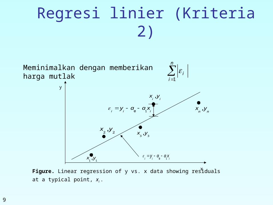
Figure. Linear regression of y vs. x data showing residuals at a typical
point, xi .

5
Contoh Kriteria 1
x y
2.0 4.0
3.0 6.0
2.0 6.0
3.0 8.0
Diberikan sejumlah titik (2,4), (3,6), (2,6) and (3,8), best fit dimodelkan dalam bentuk persamaan garis lurus
Figure. Data points for y vs. x data.
Table. Data Points
0
2
4
6
8
10
0 1 2 3 4
x
y

6
04
1
i
i
x y ypredicted ε = y - ypredicted
2.0 4.0 4.0 0.0
3.0 6.0 8.0 -2.0
2.0 6.0 4.0 2.0
3.0 8.0 8.0 0.0
Table. Residuals at each point for regression model y = 4x – 4.
Figure. Regression curve for y=4x-4, y vs. x data
0
2
4
6
8
10
0 1 2 3 4
x
y
Dengan menggunakan persamaan y=4x-4 maka diperoleh kurva regresi

7
x y ypredicted ε = y - ypredicted
2.0 4.0 6.0 -2.0
3.0 6.0 6.0 0.0
2.0 6.0 6.0 0.0
3.0 8.0 6.0 2.0
04
1
i
i
0
2
4
6
8
10
0 1 2 3 4
x
y
Table. Residuals at each point for y=6
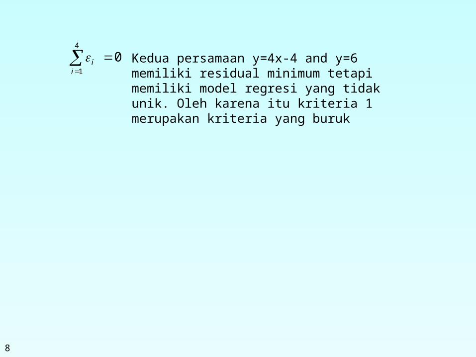
Figure. Regression curve for y=6, y vs. x data
Persamaan y=6
8
04
1
i
i Kedua persamaan y=4x-4 and y=6 memiliki residual minimum tetapi memiliki model regresi yang tidak unik. Oleh karena itu kriteria 1 merupakan kriteria yang buruk
9
Regresi linier (Kriteria 2)
x
iiixaay
10
11, yx
22, yx
33, yx
nnyx ,
iiyx ,
iiixaay
10
y
Figure. Linear regression of y vs. x data showing residuals at a typical
point, xi .
Meminimalkan dengan memberikan harga mutlak
n
ii
1

10
x y ypredicted |ε| = |y - ypredicted|
2.0 4.0 4.0 0.0
3.0 6.0 8.0 2.0
2.0 6.0 4.0 2.0
3.0 8.0 8.0 0.0
0
2
4
6
8
10
0 1 2 3 4
x
y
Table. The absolute residuals employing the y=4x-4 regression model
Figure. Regression curve for y=4x-4, y vs. x data
44
1
i
i
Dengan menggunakan persamaan y=4x-4

11
x y ypredicted |ε| = |y – ypredicted|
2.0 4.0 6.0 2.0
3.0 6.0 6.0 0.0
2.0 6.0 6.0 0.0
3.0 8.0 6.0 2.0
44
1
i
i
Table. Absolute residuals employing the y=6 model
0
2
4
6
8
10
0 1 2 3 4
xy
Figure. Regression curve for y=6, y vs. x data
Dengan persamaan y=6

12
Can you find a regression line for which
44
1
i
i and has unique
regression coefficients?
for both regression models of y=4x-4 and y=6.
The sum of the errors has been made as small as possible, that is 4, but the regression model is not unique.
Hence the above criterion of minimizing the sum of the absolute value of the residuals is also a bad criterion.
44
1
i
i

13
Least Squares Criterion
Kriteria Least Squares meminimalkan jumlah kuadrat residual dari model Persamaan.
2
110
1
2
n
iii
n
iir xaayS
x
iiixaay
10
11, yx
22, yx
33, yx
nnyx ,
iiyx ,
iiixaay
10
y
Figure. Linear regression of y vs. x data showing residuals at a typical
point, xi .
14
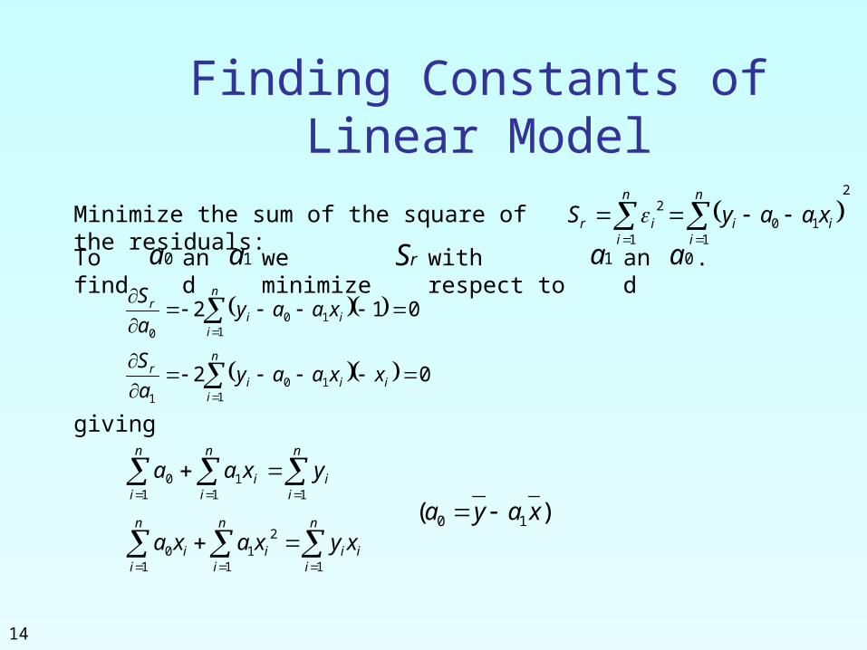
Finding Constants of Linear Model
2
110
1
2
n
iii
n
iir xaayS Minimize the sum of the square of the
residuals:To find
0121
100
n
iii
r xaaya
S
021
101
n
iiii
r xxaaya
S
giving
i
n
iii
n
ii
n
i
xyxaxa
1
2
11
10
0a and
1a we minimize
with respect to
1a 0aand
rS .
n
iii
n
i
n
i
yxaa11
11
0
)( 10 xaya

15
Finding Constants of Linear Model
0a
Solving for
2
11
2
1111
n
ii
n
ii
n
ii
n
ii
n
iii
xxn
yxyxn
a
and
2
11
2
1111
2
0
n
ii
n
ii
n
iii
n
ii
n
ii
n
ii
xxn
yxxyx
a
1aand directly yields,
)( 10 xaya

16
Example 1
The torque, T needed to turn the torsion spring of a mousetrap through an angle, is given below.
Angle, θ Torque, T
Radians N-m
0.698132 0.188224
0.959931 0.209138
1.134464 0.230052
1.570796 0.250965
1.919862 0.313707
Table: Torque vs Angle for a torsional spring
Find the constants for the model given by21 kkT
Figure. Data points for Angle vs. Torque data
0.1
0.2
0.3
0.4
0.5 1 1.5 2
θ (radians)
To
rqu
e (
N-m
)

17
Example 1 cont.
1a
The following table shows the summations needed for the calculations of the constants in the regression model.
2 T
Radians N-m Radians2 N-m-Radians
0.698132 0.188224 0.487388 0.131405
0.959931 0.209138 0.921468 0.200758
1.134464 0.230052 1.2870 0.260986
1.570796 0.250965 2.4674 0.394215
1.919862 0.313707 3.6859 0.602274
6.2831 1.1921 8.8491 1.5896
Table. Tabulation of data for calculation of important
5
1i
5nUsing equations described for
25
1
5
1
2
5
1
5
1
5
12
ii
ii
ii
ii
iii
n
TTnk
228316849185
1921128316589615
..
...
21060919 . N-m/rad
summations
0aTand
with
18
Example 1 cont.
n
TT i
i
5
1_
Use the average torque and average angle to calculate
1k
_
2
_
1 kTk
ni
i
5
1_
5
1921.1
1103842.2
5
2831.6
2566.1
Using,
)2566.1)(106091.9(103842.2 21 1101767.1 N-m
19
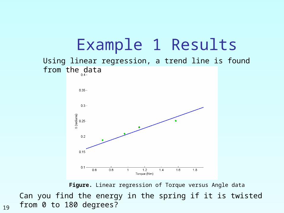
Example 1 Results
Figure. Linear regression of Torque versus Angle data
Using linear regression, a trend line is found from the data
Can you find the energy in the spring if it is twisted from 0 to 180 degrees?

20
Example 2
Strain Stress
(%) (MPa)
0 0
0.183 306
0.36 612
0.5324 917
0.702 1223
0.867 1529
1.0244 1835
1.1774 2140
1.329 2446
1.479 2752
1.5 2767
1.56 2896
To find the longitudinal modulus of composite, the following data is collected. Find the longitudinal modulus, Table. Stress vs. Strain data
E using the regression model E and the sum of the square of
the
0.0E+00
1.0E+09
2.0E+09
3.0E+09
0 0.005 0.01 0.015 0.02
Strain, ε (m/m)
Str
ess,
σ (
Pa)
residuals.
Figure. Data points for Stress vs. Strain data

21
Example 2 cont.
iii E Residual at each point is given by
The sum of the square of the residuals then is
n
iirS
1
2
n
iii E
1
2
0)(21
i
n
iii
r EE
S
Differentiate with respect to
E
n
ii
n
iii
E
1
2
1
Therefore

22
Example 2 cont.
i ε σ ε 2 εσ
1 0.0000 0.0000 0.0000 0.0000
2 1.8300×10⁻³ 3.0600×10⁸ 3.3489×10⁻⁶ 5.5998×10⁵
3 3.6000×10⁻³ 6.1200×10⁸ 1.2960×10⁻⁵ 2.2032×10⁶
4 5.3240×10⁻³ 9.1700×10⁸ 2.8345×10⁻⁵ 4.8821×10⁶
5 7.0200×10⁻³ 1.2230×10⁹ 4.9280×10⁻⁵ 8.5855×10⁶
6 8.6700×10⁻³ 1.5290×10⁹ 7.5169×10⁻⁵ 1.3256×10⁷
7 1.0244×10⁻² 1.8350×10⁹ 1.0494×10⁻⁴ 1.8798×10⁷
8 1.1774×10⁻² 2.1400×10⁹ 1.3863×10⁻⁴ 2.5196×10⁷
9 1.3290×10⁻² 2.4460×10⁹ 1.7662×10⁻⁴ 3.2507×10⁷
10 1.4790×10⁻² 2.7520×10⁹ 2.1874×10⁻⁴ 4.0702×10⁷
11 1.5000×10⁻² 2.7670×10⁹ 2.2500×10⁻⁴ 4.1505×10⁷
12 1.5600×10⁻² 2.8960×10⁹ 2.4336×10⁻⁴ 4.5178×10⁷
1.2764×10⁻³ 2.3337×10⁸
Table. Summation data for regression model
12
1i
12
1
32 102764.1i
i
With
and
12
1
8103337.2i
ii
Using
12
1
2
12
1
ii
iii
E
3
8
102764.1
103337.2
GPa84.182

23
Example 2 Results 84.182The
equation
Figure. Linear regression for Stress vs. Strain data
describes the data.

REGRESI NON LINIER

Nonlinear Regression
)( bxaey
)( baxy
xb
axy
Some popular nonlinear regression models:
1. Exponential model:2. Power model:
3. Saturation growth model:4. Polynomial model: )( 10
mmxa...xaay
25

Nonlinear Regression
Given n data points
),( , ... ),,(),,( 2211 nn yxyx yx best fit )(xfy
to the data, where
)(xf is a nonlinear function of
x .
Figure. Nonlinear regression model for discrete y vs. x data
)(xfy
),(nn
yx
),(11
yx
),(22
yx
),(ii
yx
)(ii
xfy
26

RegressionExponential Model
27

Exponential Model),( , ... ),,(),,( 2211 nn yxyx yxGive
nbest fit
bxaey to the data.
Figure. Exponential model of nonlinear regression for y vs. x data
bxaey
),(nn
yx
),(11
yx
),(22
yx
),(ii
yx
)(ii
xfy
28

Finding Constants of Exponential Model
n
i
bx
ir iaeyS
1
2
The sum of the square of the residuals is defined as
Differentiate with respect to a and b
021
ii bxn
i
bxi
r eaeya
S
021
ii bxi
n
i
bxi
r eaxaeyb
S
29

Finding Constants of Exponential Model
Rewriting the equations, we obtain
01
2
1
n
i
bxn
i
bxi
ii eaey
01
2
1
n
i
bxi
n
i
bxii
ii exaexy
30

Finding constants of Exponential Model
Substituting a back into the previous equation
01
2
1
2
1
1
n
i
bxin
i
bx
bxn
ii
bxi
n
ii
i
i
i
i exe
eyexy
The constant b can be found through numerical methods such as bisection method.
n
i
bx
n
i
bxi
i
i
e
eya
1
2
1
Solving the first equation for a yields
31

Example 1-Exponential Model
t(hrs) 0 1 3 5 7 9
1.000 0.891 0.708 0.562 0.447 0.355
Many patients get concerned when a test involves injection of a radioactive material. For example for scanning a gallbladder, a few drops of Technetium-99m isotope is used. Half of the techritium-99m would be gone in about 6 hours. It, however, takes about 24 hours for the radiation levels to reach what we are exposed to in day-to-day activities. Below is given the relative intensity of radiation as a function of time.
Table. Relative intensity of radiation as a function of time.
32

Example 1-Exponential Model cont.
Find: a) The value of the regression
constants A an
db) The half-life of Technium-99m
c) Radiation intensity after 24 hours
The relative intensity is related to time by the equation tAe
33

Plot of data
34

Constants of the Model
The value of λ is found by solving the nonlinear equation
01
2
1
2
1
1
n
i
tin
i
t
n
i
ti
ti
n
ii
i
i
i
i ete
eetf
n
i
t
n
i
ti
i
i
e
eA
1
2
1
tAe
35

Setting up the Equation in MATLAB
01
2
1
2
1
1
n
i
tin
i
t
n
i
ti
ti
n
ii
i
i
i
i ete
eetf
t (hrs) 0 1 3 5 7 9
γ 1.000
0.891
0.708
0.562
0.447
0.35536
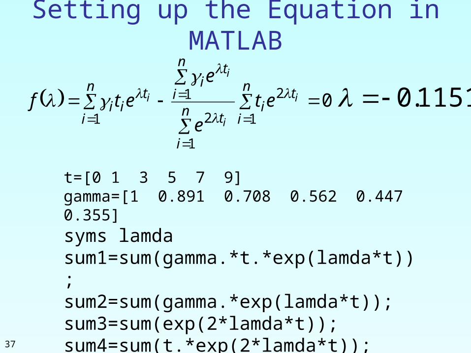
Setting up the Equation in MATLAB
01
2
1
2
1
1
n
i
tin
i
t
n
i
ti
ti
n
ii
i
i
i
i ete
eetf
t=[0 1 3 5 7 9]gamma=[1 0.891 0.708 0.562 0.447 0.355]syms lamdasum1=sum(gamma.*t.*exp(lamda*t));sum2=sum(gamma.*exp(lamda*t));sum3=sum(exp(2*lamda*t));sum4=sum(t.*exp(2*lamda*t));f=sum1-sum2/sum3*sum4;
1151.0
37

Calculating the Other Constant
The value of A can now be calculated
6
1
2
6
1
i
t
i
ti
i
i
e
eA
9998.0
The exponential regression model then is te 1151.0 9998.0
38

Plot of data and regression curve
te 1151.0 9998.0
39

Relative Intensity After 24 hrs
The relative intensity of radiation after 24 hours 241151.09998.0 e
2103160.6 This result implies that only
%317.61009998.0
10316.6 2
radioactive intensity is left after 24 hours.
40

Homework• What is the half-life of technetium
99m isotope?• Compare the constants of this
regression model with the one where the data is transformed.
• Write a program in the language of your choice to find the constants of the model.
41

Polynomial Model),( , ... ),,(),,( 2211 nn yxyx yxGiven best
fit
m
mxa...xaay
10
)2( nm to a given data set.
Figure. Polynomial model for nonlinear regression of y vs. x data
m
mxaxaay
10
),(nn
yx
),(11
yx
),(22
yx
),(ii
yx
)(ii
xfy
42

Polynomial Model cont.The residual at each data point is given by
mimiii xaxaayE ...10
The sum of the square of the residuals then is
n
i
mimii
n
iir
xaxaay
ES
1
2
10
1
2
...
43

Polynomial Model cont.To find the constants of the polynomial model, we set the derivatives with respect to ia wher
e
0)(....2
0)(....2
0)1(....2
110
110
1
110
0
mi
n
i
mimii
m
r
i
n
i
mimii
r
n
i
mimii
r
xxaxaaya
S
xxaxaaya
S
xaxaaya
S
,,1 mi equal to zero.
44

Polynomial Model cont.These equations in matrix form are
given by
n
ii
mi
n
iii
n
ii
mn
i
mi
n
i
mi
n
i
mi
n
i
mi
n
ii
n
ii
n
i
mi
n
ii
yx
yx
y
a
a
a
xxx
xxx
xxn
1
1
1
1
0
1
2
1
1
1
1
1
1
2
1
11
......
...
...........
...
...
The above equations are then solved for
maaa ,,, 10
45

Example 2-Polynomial Model
Temperature, T(oF)
Coefficient of thermal
expansion, α (in/in/oF)
80 6.47×10⁻⁶
40 6.24×10⁻⁶
−40 5.72×10⁻⁶
−120 5.09×10⁻⁶
−200 4.30×10⁻⁶
−280 3.33×10⁻⁶
−340 2.45×10⁻⁶
Regress the thermal expansion coefficient vs. temperature data to a second order polynomial.
1.00E-06
2.00E-06
3.00E-06
4.00E-06
5.00E-06
6.00E-06
7.00E-06
-400 -300 -200 -100 0 100 200
Temperature, oF
Th
erm
al e
xpan
sio
n c
oef
fici
ent,
α
(in
/in
/oF
)
Table. Data points for temperature vs
Figure. Data points for thermal expansion coefficient vs temperature.
α
46

Example 2-Polynomial Model cont.
2210 TaTaaα
We are to fit the data to the polynomial regression model
n
iii
n
iii
n
ii
n
ii
n
ii
n
ii
n
ii
n
ii
n
ii
n
ii
n
ii
T
T
a
a
a
TTT
TTT
TTn
1
2
1
1
2
1
0
1
4
1
3
1
2
1
3
1
2
1
1
2
1
The coefficients
210 , a,aa are found by differentiating the sum of thesquare of the residuals with respect to each variable and
setting thevalues equal to zero to obtain
47

Example 2-Polynomial Model cont.
The necessary summations are as follows
Temperature, T(oF)
Coefficient of thermal expansion,
α (in/in/oF)
80 6.47×10⁻⁶
40 6.24×10⁻⁶
−40 5.72×10⁻⁶
−120 5.09×10⁻⁶
−200 4.30×10⁻⁶
−280 3.33×10⁻⁶
−340 2.45×10⁻⁶
Table. Data points for temperature vs.
α 57
1
2 105580.2 i
iT
77
1
3 100472.7 i
iT
107
1
4 101363.2
i
iT
57
1
103600.3
i
i
37
1
106978.2
i
iiT
17
1
2 105013.8
i
iiT
48

Example 2-Polynomial Model cont.
1
3
5
2
1
0
1075
752
52
105013.8
106978.2
103600.3
101363.2100472.7105800.2
100472.7105800.210600.8
105800.2106000.80000.7
a
a
a
Using these summations, we can now calculate
210 , a,aa
Solving the above system of simultaneous linear equations we have
11
9
6
2
1
0
102218.1
102782.6
100217.6
a
a
a
The polynomial regression model is then
21196
2210
T101.2218T106.2782106.0217
α
TaTaa
49
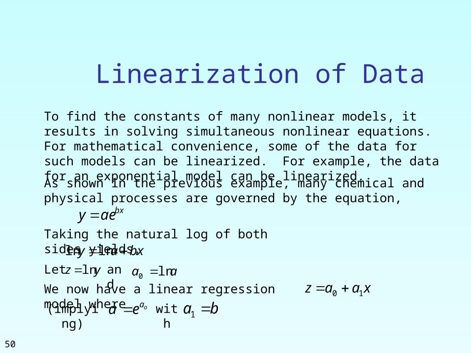
Linearization of DataTo find the constants of many nonlinear models, it results in solving simultaneous nonlinear equations. For mathematical convenience, some of the data for such models can be linearized. For example, the data for an exponential model can be linearized.As shown in the previous example, many chemical and physical processes are governed by the equation,
bxaey Taking the natural log of both sides yields, bxay lnln
Let yz ln and
aa ln0
(implying)
oaea with
ba 1
We now have a linear regression model where
xaaz 10
50

Linearization of data cont.Using linear model regression methods,
_
1
_
0
1
2
1
2
11 11
xaza
xxn
zxzxna
n
i
n
iii
n
ii
n
i
n
iiii
Once 1,aao are found, the original constants of the model are found as
0
1
aea
ab
51

Example 3-Linearization of data
t(hrs) 0 1 3 5 7 9
1.000 0.891 0.708 0.562 0.447 0.355
Many patients get concerned when a test involves injection of a radioactive material. For example for scanning a gallbladder, a few drops of Technetium-99m isotope is used. Half of the technetium-99m would be gone in about 6 hours. It, however, takes about 24 hours for the radiation levels to reach what we are exposed to in day-to-day activities. Below is given the relative intensity of radiation as a function of time.
Table. Relative intensity of radiation as a function
of time
0
0.5
1
0 5 10
Rel
ativ
e in
ten
sity
of r
adia
tio
n, γ
Time t, (hours)
Figure. Data points of relative radiation intensity vs. time
52

Example 3-Linearization of data cont.
Find: a) The value of the regression
constants A an
db) The half-life of Technium-99m
c) Radiation intensity after 24 hours
The relative intensity is related to time by the equation tAe
53

Example 3-Linearization of data cont.
tAe Exponential model given as,
tA lnln
Assuming
lnz , Aao ln and 1a we obtaintaaz
10
This is a linear relationship between
z and t
54

Example 3-Linearization of data cont.
Using this linear relationship, we can calculate
10 , aa
n
i
n
ii
n
ii
n
i
n
iiii
ttn
ztztna
1
2
1
2
1
11 1
1
and
taza 10
where
1a
0a
eA
55

Example 3-Linearization of Data cont.
123456
013579
10.8910.7080.5620.4470.355
0.00000−0.11541−0.34531−0.57625−0.80520−1.0356
0.0000−0.11541−1.0359−2.8813−5.6364−9.3207
0.00001.00009.000025.00049.00081.000
25.000 −2.8778 −18.990 165.00
Summations for data linearization are as follows
Table. Summation data for linearization of data model
i it i iiz ln ii
zt 2it
With 6n
000.256
1
i
it
6
1
8778.2i
iz
6
1
990.18i
iizt
00.1656
1
2 i
it
56
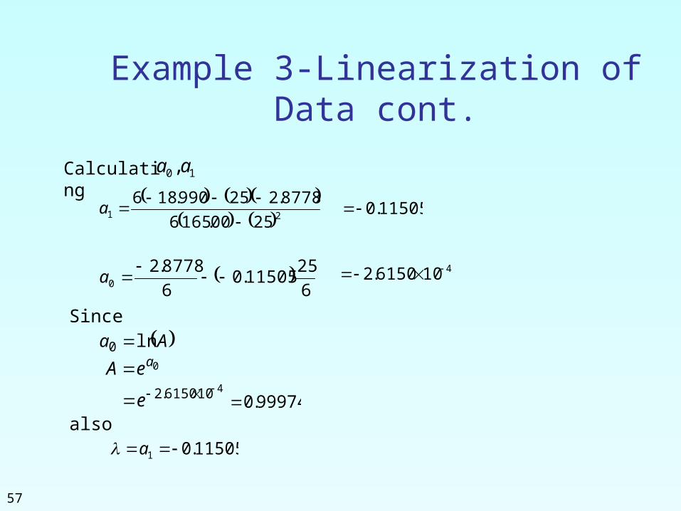
Example 3-Linearization of Data cont.
Calculating 10 ,aa
21
2500.1656
8778.225990.186
a 11505.0
6
2511505.0
6
8778.20
a4106150.2
Since Aa ln0 0aeA
4106150.2 e 99974.0
11505.01 aalso
57
Example 3-Linearization of Data cont.
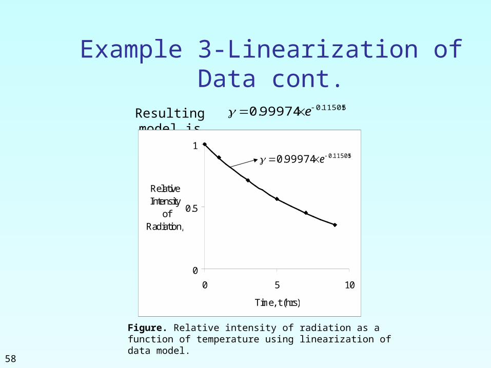
Resulting model is
te 11505.099974.0
0
0.5
1
0 5 10
Time, t (hrs)
Relative Intensity
of Radiation,
te 11505.099974.0
Figure. Relative intensity of radiation as a function of temperature using linearization of data model.
58

Example 3-Linearization of Data cont.
The regression formula is thente 11505.099974.0
b) Half life of Technetium 99 is when02
1
t
hours.t
.t.
.e
e.e.
t.
.t.
02486
50ln115050
50
9997402
1999740
115080
0115050115050
59

Example 3-Linearization of Data cont.
c) The relative intensity of radiation after 24 hours is then 2411505.099974.0 e
063200.0This implies that only
%3216.610099983.0
103200.6 2
of the radioactive
material is left after 24 hours.
60

Comparison Comparison of exponential model with and without data linearization:
With data linearization(Example 3)
Without data linearization(Example 1)
A 0.99974 0.99983
λ −0.11505 −0.11508
Half-Life (hrs) 6.0248 6.0232
Relative intensity after 24 hrs.
6.3200×10⁻² 6.3160×10⁻²
Table. Comparison for exponential model with and without data linearization.
The values are very similar so data linearization was suitable to find the constants of the nonlinear exponential model in this case.
61
62
ADEQUACY OF REGRESSION MODELS

Data
-350 -300 -250 -200 -150 -100 -50 0 50 1002
2.5
3
3.5
4
4.5
5
5.5
6
6.5
x
yy vs x
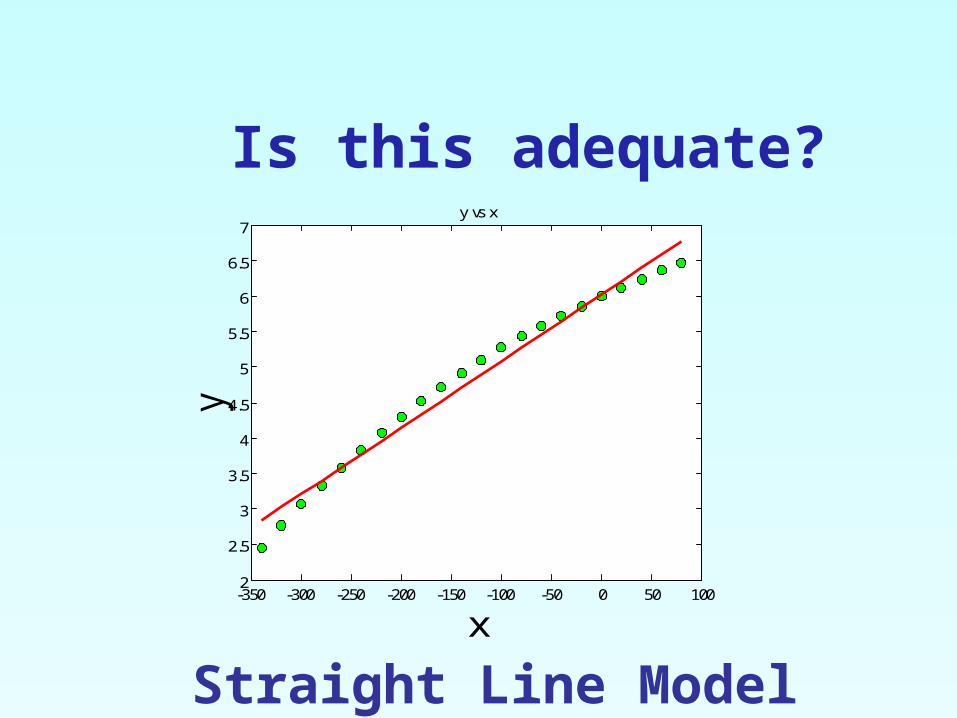
Is this adequate?
-350 -300 -250 -200 -150 -100 -50 0 50 1002
2.5
3
3.5
4
4.5
5
5.5
6
6.5
7
x
yy vs x
Straight Line Model
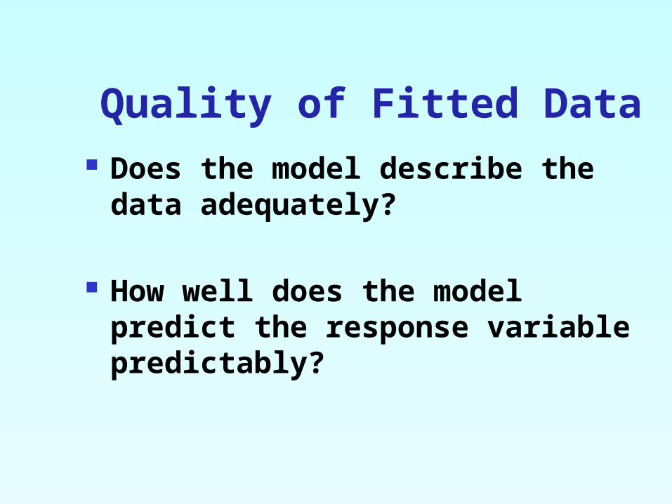
Quality of Fitted Data Does the model describe the
data adequately?
How well does the model predict the response variable predictably?

Linear Regression Models
Limit our discussion to adequacy of straight-line regression models

Four checks
1. Plot the data and the model.2. Find standard error of
estimate.3. Calculate the coefficient of
determination.4. Check if the model meets the
assumption of random errors.

Example: Check the adequacy of the straight line model for given data
T
(F)
α (μin/in/F)
-340 2.45
-260 3.58
-180 4.52
-100 5.28
-20 5.86
60 6.36
Taa 10

1. Plot the data and the model

Data and model
T
(F)
α (μin/in/F)
-340 2.45
-260 3.58
-180 4.52
-100 5.28
-20 5.86
60 6.36-350 -300 -250 -200 -150 -100 -50 0 50 1002
2.5
3
3.5
4
4.5
5
5.5
6
6.5
7
T
TT 0096964.00325.6)(
2. Find the standard error of estimate

Standard error of estimate
2/
n
Ss r
T
n
iiir TaaS
1
210 )(

Standard Error of Estimate
-340-260-180-100-2060
2.453.584.525.285.866.36
2.73573.51144.28715.06295.83866.6143
-0.285710.0685710.232860.21714
0.021429-0.25429
iT i iTaa 10 ii Taa 10
TT 0096964.00325.6)(

Standard Error of Estimate
25283.0rS
2/
n
Ss r
T
26
25283.0
25141.0

Standard Error of Estimate
T
ii
s
Taa
/
10 ResidualScaled
-350 -300 -250 -200 -150 -100 -50 0 50 1002
3
4
5
6
7
8
T

Scaled Residuals
T
ii
s
Taa
/
10 ResidualScaled
Estimateof Error Standard
Residual ResidualScaled
95% of the scaled residuals need to be in [-2,2]

Scaled Residuals
Ti αi ResidualScaled
Residual
-340-260-180-100-2060
2.453.584.525.285.866.36
-0.285710.0685710.232860.217140.021429-0.25429
-1.13640.272750.926220.863690.085235-1.0115
25141.0/ Ts

3. Find the coefficient of determination

Coefficient of determination
n
iiir TaaS
1
210
n
iitS
1
2
t
rt
S
SSr
2

Sum of square of residuals between data and mean
n
iitS
1
2
11, yx
33 , yx 22 , yx
),( nn yx
ii yx ,y
x
_
yy _
yy

Sum of square of residuals between observed and
predicted
n
iiir TaaS
1
210
11, yx
33 , yx
22 , yx
),( nn yx
ii yx ,
iii xaayE 10
y
x

Limits of Coefficient of Determination
t
rt
S
SSr
2
10 2 r
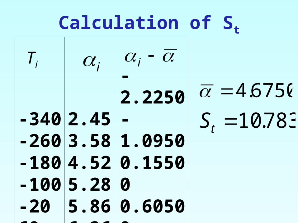
Calculation of St
-340-260-180-100-2060
2.453.584.525.285.866.36
-2.2250-1.09500.155000.605001.18501.6850
iTi i
783.10tS
6750.4

Calculation of Sr
-340-260-180-100-2060
2.453.584.525.285.866.36
2.73573.51144.28715.06295.83866.6143
-0.285710.0685710.232860.21714
0.021429-0.25429
iT i iTaa 10 ii Taa 10
25283.0rS
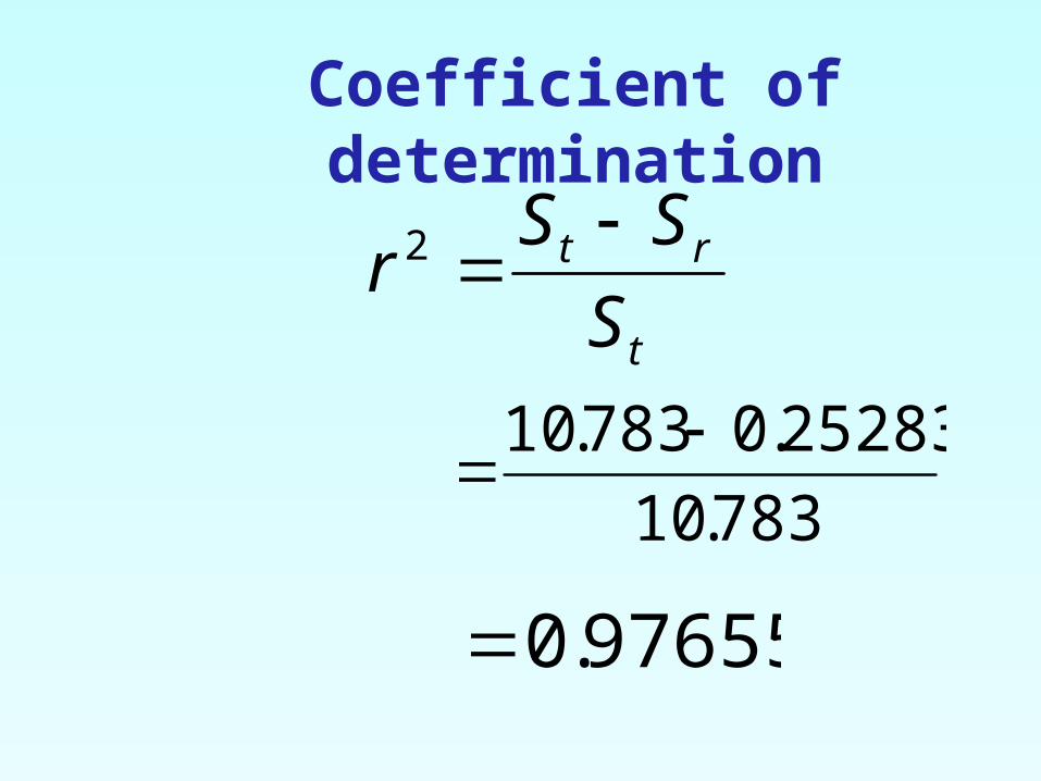
Coefficient of determination
t
rt
S
SSr
2
783.10
25283.0783.10
97655.0

Caution in use of r2
Increase in spread of regressor variable (x) in y vs. x increases r2
Large regression slope artificially yields high r2
Large r2 does not measure appropriateness of the linear model
Large r2 does not imply regression model will predict accurately

Final Exam Grade

Final Exam Grade vs Pre-Req GPA
4. Model meets assumption of random errors

Model meets assumption of random errors
Residuals are negative as well as positive
Variation of residuals as a function of the independent variable is random
Residuals follow a normal distribution
There is no autocorrelation between the data points.

Therm exp coeff vs temperature
T α
60 6.36
40 6.24
20 6.12
0 6.00
-20 5.86
-40 5.72
-60 5.58
-80 5.43
T α
-100 5.28
-120 5.09
-140 4.91
-160 4.72
-180 4.52
-200 4.30
-220 4.08
-240 3.83
T α
-280 3.33
-300 3.07
-320 2.76
-340 2.45

Data and model
-350 -300 -250 -200 -150 -100 -50 0 50 1002
2.5
3
3.5
4
4.5
5
5.5
6
6.5
7
T
T0093868.00248.6

Plot of Residuals
-350 -300 -250 -200 -150 -100 -50 0 50 100-0.4
-0.3
-0.2
-0.1
0
0.1
0.2
0.3
T
Res
idua
l

Histograms of Residuals

Check for Autocorrelation
Find the number of times, q the sign of the residual changes for the n data points.
If (n-1)/2-√(n-1) ≤q≤ (n-1)/2+√(n-1), you most likely do not have an autocorrelation.
1222
122122
2
)122(
q
083.159174.5 q

Is there autocorrelation?
083.159174.5 q
-350 -300 -250 -200 -150 -100 -50 0 50 100-0.4
-0.3
-0.2
-0.1
0
0.1
0.2
0.3
T
Residu
al
y vs x fit and residuals
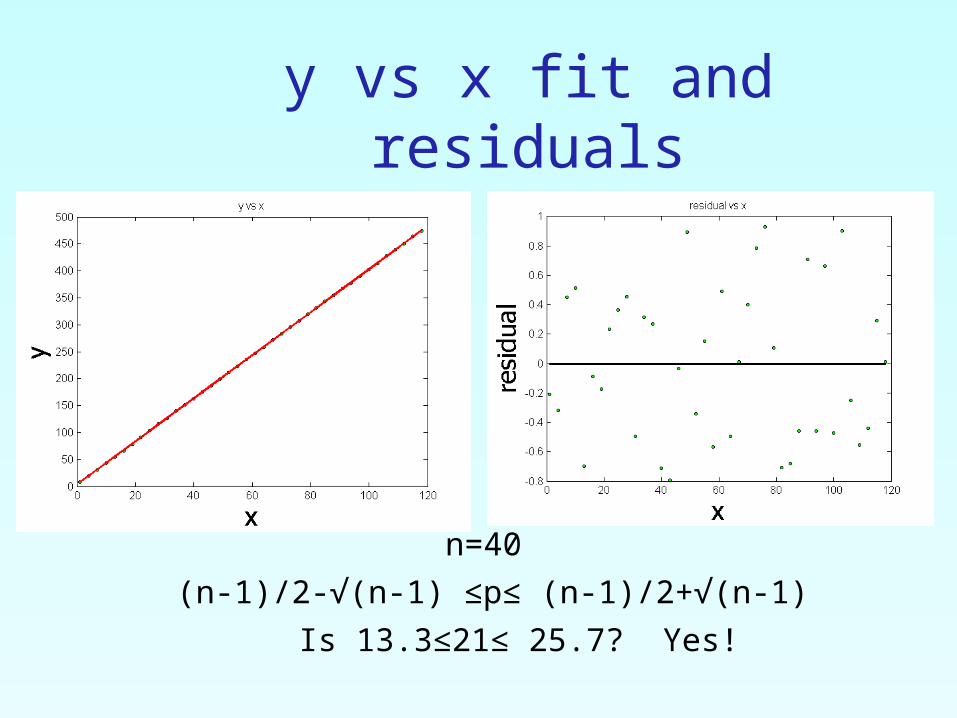
n=40
Is 13.3≤21≤ 25.7? Yes!
(n-1)/2-√(n-1) ≤p≤ (n-1)/2+√(n-1)

y vs x fit and residuals
(n-1)/2-√(n-1) ≤p≤ (n-1)/2+√(n-1)
Is 13.3≤2≤ 25.7? No!
n=40

What polynomial model to choose if one needs to be
chosen?

First Order of Polynomial
-350 -300 -250 -200 -150 -100 -50 0 50 1002
2.5
3
3.5
4
4.5
5
5.5
6
6.5
7x 10
-6 Polynomial Regression of order 1
x
y =
a0+
a 1*x+
a 2*x2 +
....
.+a m
*xm

Second Order Polynomial
-350 -300 -250 -200 -150 -100 -50 0 50 1002
2.5
3
3.5
4
4.5
5
5.5
6
6.5
7x 10
-6 Polynomial Regression of order 2
x
y =
a0+
a 1*x+
a 2*x2 +
....
.+a m
*xm

Which model to choose?
-350 -300 -250 -200 -150 -100 -50 0 50 1002
2.5
3
3.5
4
4.5
5
5.5
6
6.5
7
x
yy vs x

Optimum Polynomial
0 1 2 3 4 5 60
1
2
3
4
5
x 10-14 Optimum Order of Polynomial
Order of Polynomial, m
Sr
[n-(
m+
1)]

Effect of an Outlier

Effect of Outlier
y = 2x
R2 = 1
0
5
10
15
20
25
0 2 4 6 8 10 12

Effect of Outlier
y = 3.2727x - 5.0909
R2 = 0.6879
-10
0
10
20
30
40
50
60
0 2 4 6 8 10 12