forecasting -...
TRANSCRIPT

FORECASTING FORECASTING DR. MOHAMMAD ABDUL MUKHYI, SE., MM
6/3/2008 1

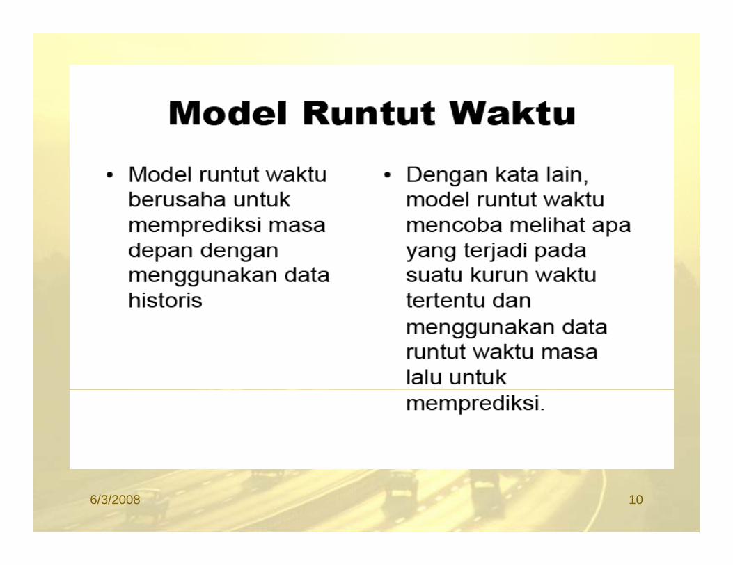
Apa Arti Runtut Waktu?• Data runtut waktu (time series) merupakan data yang
dikumpulkan, dicatat, atau diobservasi sepanjangp , , p j gwaktu secara berurutan
• Periode waktu dapat tahun, kuartal, bulan, minggu, dan dibeberapa kasus hari atau jamdan dibeberapa kasus hari atau jam.
• Runtut waktu dianalisis untuk menemukan polavariasi masa lalu yang dapat dipergunakan untuk: y g p p g(1) memprakirakan nilai masa depan dan membantu
dalam manajemen operasi bisnis; (2) membuat perencanaan bahan baku, fasilitas
produksi, dan jumlah staf guna memenuhipermintaan dimasa mendatang. pe taa d asa e data g
6/3/2008 2

Mengapa Mempelajari Analisisg p p jRuntut Waktu?
K d ti d t t t kt kKarena dengan mengamati data runtut waktu akanterlihat empat komponen yang mempengaruhi suatupola data masa lalu dan sekarang, yang cenderungberulang dimasa mendatang
6/3/2008 3
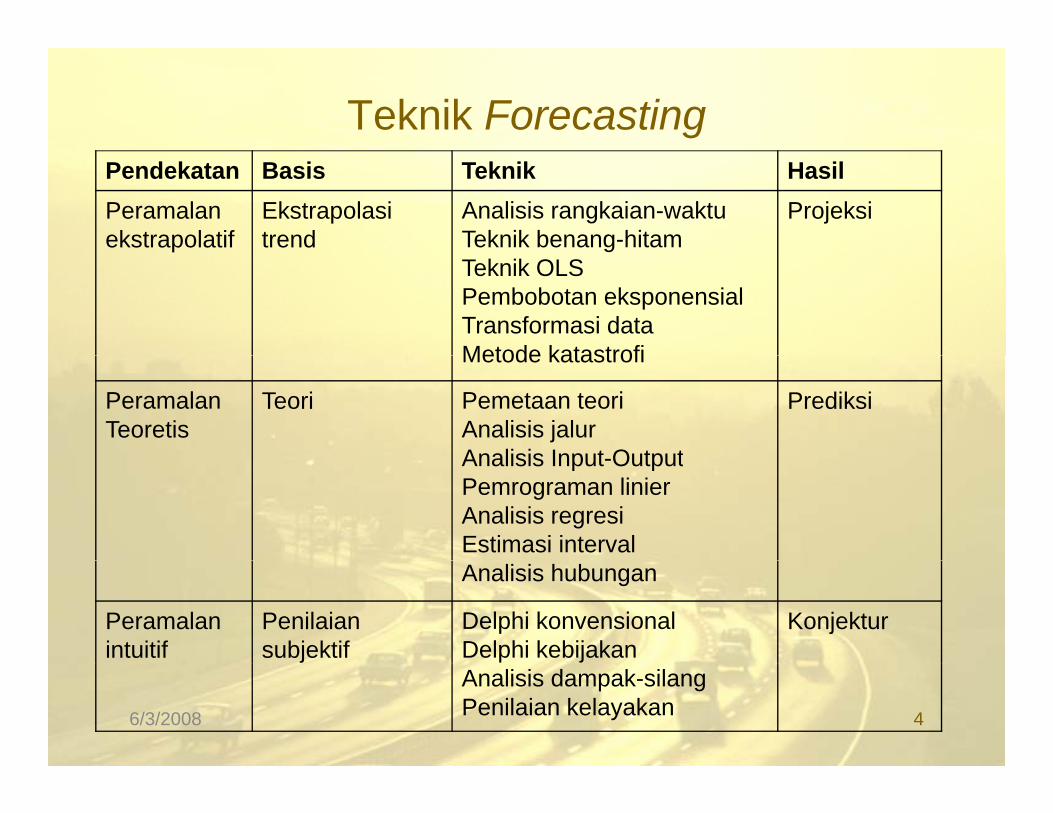
Teknik ForecastingPendekatan Basis Teknik HasilPeramalan ekstrapolatif
Ekstrapolasi trend
Analisis rangkaian-waktuTeknik benang-hitam
Projeksi
Teknik OLSPembobotan eksponensialTransformasi dataMetode katastrofiMetode katastrofi
PeramalanTeoretis
Teori Pemetaan teoriAnalisis jalurAnalisis Input Output
Prediksi
Analisis Input-OutputPemrograman linierAnalisis regresiEstimasi intervalAnalisis hubungan
Peramalan intuitif
Penilaian subjektif
Delphi konvensionalDelphi kebijakan
Konjektur
Analisis dampak-silangPenilaian kelayakan6/3/2008 4

Asumsi Peramalan Ekstrapolatif1. Keajegan (persistence): Pola yang terjadi di
masa lalu akan tetap terjadi di masa mendatang. Mis: jika konsumsi energi di masamendatang. Mis: jika konsumsi energi di masa lalu meningkat, ia akan selalu meningkat di masa depan.
2 Keteraturan (regularity): Variasi di masa lalu2. Keteraturan (regularity): Variasi di masa lalu akan secara teratur muncul di masa depan. Mis: jika banjir besar di Jakarta terjadi setiap 16 tah n sekali pola g sama akan terjadi lagi16 tahun sekali, pola yg sama akan terjadi lagi.
3. Keandalan (reliability) dan kesahihan (validity) data: Ketepatan ramalan tergantung kepada p g g pkeandalan dan kesahihan data yg tersedia. Mis: data ttg laporan kejahatan seringkali tidak sesuai dg insiden kejahatan yg sesungguhnya,sesuai dg insiden kejahatan yg sesungguhnya, data ttg gaji bukan merupakan ukuran tepat dari pendapatan masyarakat.6/3/2008 5
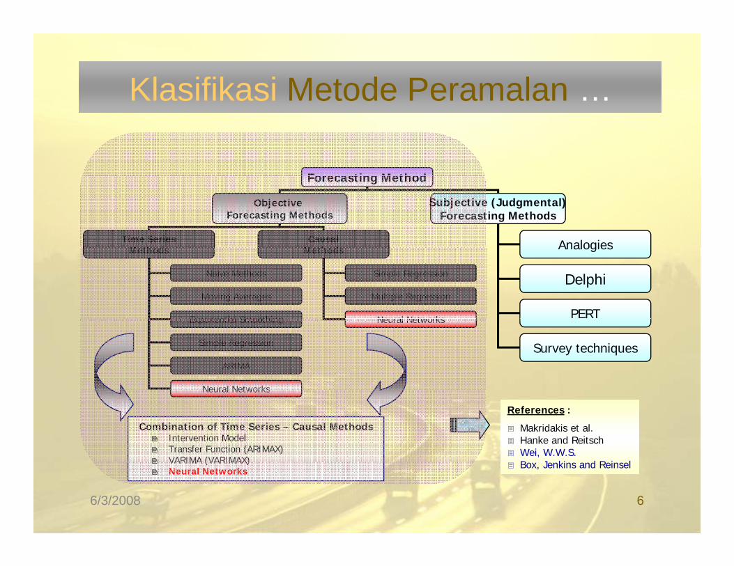
Klasifikasi Metode Peramalan …
Forecasting MethodForecasting Method
Objective Forecasting Methods
Subjective (Judgmental)Forecasting Methods
Time SeriesM th d
CausalM th d AnalogiesMethods Methods Analogies
Delphi
PERT
Simple Regression
Multiple Regression
Neural Networks
Naïve Methods
Moving Averages
Exponential Smoothing
Survey techniques
Neural NetworksExponential Smoothing
Simple Regression
ARIMA
Neural NetworksNeural Networks
Combination of Time Series – Causal MethodsIntervention ModelTransfer Function (ARIMAX)VARIMA (VARIMAX)
References :
Makridakis et al. Hanke and ReitschWei, W.W.S. B J ki d R i lVARIMA (VARIMAX)
Neural NetworksBox, Jenkins and Reinsel
6/3/2008 6
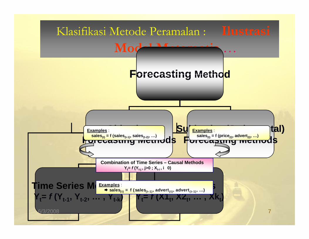
Klasifikasi Metode Peramalan : Ilustrasi M d l M iModel Matematis …
Forecasting MethodForecasting MethodForecasting MethodForecasting Method
Objective Subjective (Judgmental)Examples :� l f ( l l )
Examples :� l f ( i d t )
Objective Subjective (Judgmental)Examples :� l f ( l l )
Examples :� l f ( i d t )Forecasting Methods Forecasting Methods� sales(t) = f (sales(t-1), sales(t-2), …) � sales(t) = f (price(t), advert(t), …)
Combination of Time Series – Causal Methods
Forecasting Methods Forecasting Methods� sales(t) = f (sales(t-1), sales(t-2), …) � sales(t) = f (price(t), advert(t), …)
Combination of Time Series – Causal Methods
Time Series MethodsY = f (Y Y Y )
Causal MethodsY = f (X1 X2 Xk )
Yt= f (Yt-j , j>0 ; Xt-i , i�0)
Time Series MethodsY = f (Y Y Y )
Causal MethodsY = f (X1 X2 Xk )
Yt= f (Yt-j , j>0 ; Xt-i , i�0)
Examples :sales(t) = f (sales(t-1), advert(t), advert(t-1), …)
Yt= f (Yt-1, Yt-2, … , Yt-k) Yt= f (X1t, X2t, … , Xkt)Yt= f (Yt-1, Yt-2, … , Yt-k) Yt= f (X1t, X2t, … , Xkt)6/3/2008 7

Klasifikasi Model Time Series : Berdasarkan B t k t F iTIME SERIES MODELS
LINEARTime Series Models
NONLINEARTime Series Models
Bentuk atau Fungsi …
Time Series Models Time Series Models
ARIMA Box-Jenkins Models from time series theory� nonlinear autoregressive, etc ...
Flexible statistical parametric models � neural network model, etc ...Intervention Model
State-dependent, time-varying para-meter and long-memory modelsTransfer Function (ARIMAX)
Nonparametric modelsVARIMA (VARIMAX)
Models from economic theoryReferences :
Timo Terasvirta, Dag Tjostheim and Clive W.J. Granger, (1994) “Aspects of Modelling Nonlinear Time Series” Handbook of Econometrics, Volume IV, Chapter 48. Edited by R.F. Engle and D.I. McFadden
6/3/2008 8
6/3/2008 9
6/3/2008 10

6/3/2008 11

6/3/2008 12

6/3/2008 13
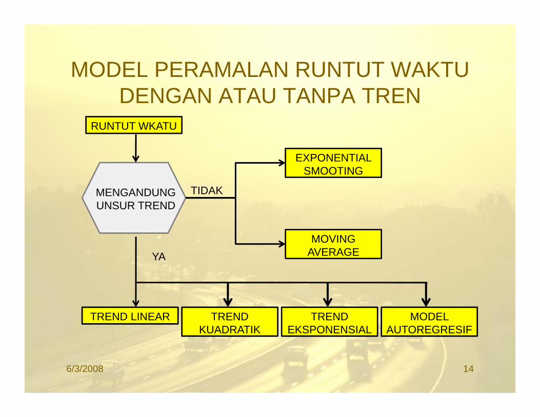
MODEL PERAMALAN RUNTUT WAKTU O U U UDENGAN ATAU TANPA TREN
RUNTUT WKATUU U U
EXPONENTIAL SMOOTING
MENGANDUNG UNSUR TREND
MOVING
TIDAK
MOVING AVERAGEYA
MODEL AUTOREGRESIF
TREND EKSPONENSIAL
TREND KUADRATIK
TREND LINEAR
6/3/2008 14

Empat komponen yang ditemukan dalam analisisruntut waktu adalah:1. Trend, yaitu komponen jangka panjang yang
mendasari pertumbuhan (atau penurunan) suatu data p ( p )runtut waktu.
2. Siklikal (cyclical), yaitu suatu pola fluktuasi atausiklus dari data runtut waktu akibat perubahansiklus dari data runtut waktu akibat perubahankondisi ekonomi.
3. Musiman (seasonal), yaitu fluktuasi musiman yang i dij i d d t k t l b l tsering dijumpai pada data kuartalan, bulanan atau
mingguan.4. Tak beraturan (irregular), yaitu pola acak yang
disebabkan oleh peristiwa yang tidak dapat diprediksiatau tidak beraturan, seperti perang, pemogokan, pemilu, atau longsor maupun bencana alam lainnyap , g p y
6/3/2008 15

General of Time Series Patterns …
STime Series Patterns
Stationer Trend Effect Seasonal Effect Cyclic Effect
Nonseasonal Nonstationary models
Seasonal and Multiplicative models
Intervention models
Nonseasonal Stationary models y py
6/3/2008 16
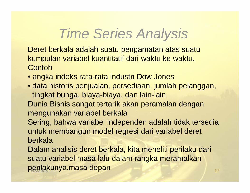
Time Series AnalysisTime Series AnalysisDeret berkala adalah suatu pengamatan atas suatukumpulan variabel kuantitatif dari waktu ke waktukumpulan variabel kuantitatif dari waktu ke waktu.Contoh• angka indeks rata-rata industri Dow Jones
data historis penjualan persediaan jumlah pelanggan• data historis penjualan, persediaan, jumlah pelanggan, tingkat bunga, biaya-biaya, dan lain-lain
Dunia Bisnis sangat tertarik akan peramalan denganmengunakan variabel berkalaSering, bahwa variabel independen adalah tidak tersediauntuk membangun model regresi dari variabel deretuntuk membangun model regresi dari variabel deretberkalaDalam analisis deret berkala, kita meneliti perilaku darisuatu variabel masa lalu dalam rangka meramalkansuatu variabel masa lalu dalam rangka meramalkanperilakunya.masa depan6/3/2008 17

Pola dataPola dataGeneral Time Series “PATTERN”
St tiStationerTrend (linear or nonlinear) Seasonal (additive or multiplicative)Cyclic Calendar Variation
6/3/2008 18

Pendekatan Analisis Deret BerkalaPendekatan Analisis Deret BerkalaAda banyak teknik deret berkala.I i bi ki t k t h i t k ikIni biasanya mungkin untuk mengetahui teknik mana yang terbaik untuk data tertentu.Biasanya mencoba beberapa teknik berbeda danmemilih salah satu terbaik.Untuk menjadi suatu model deret berkala yang efektif, ini harus menyediakan beberapa teknikderet berkala diini harus menyediakan beberapa teknikderet berkala didalam “ tool box.”
6/3/2008 19

Measuring Accuracy• We need a way to compare different time series• We need a way to compare different time series
techniques for a given data set.• Four common techniques are the:
– mean absolute deviation, MAD = Y Yi i
i
n
n−
=∑
$
1
– mean absolute percent error,
i=1
∑−n ii
n Y
YY100 = MAPE
– the mean square error,( )
MSE =Y Yi i
n −∑
$ 2=i in 1 Y
the mean square error,
– root mean square error.
MSE i n=∑
1
MSERMSE =
We will focus on the MSE.6/3/2008 20
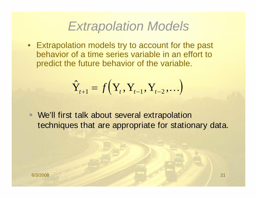
Extrapolation Models• Extrapolation models try to account for the past
behavior of a time series variable in an effort to di t th f t b h i f th i blpredict the future behavior of the variable.
( )$Y Y Y Yf ( ), , ,Y Y Y Yt t t tf+ − −=1 1 2 K
’ll f lk b l lWe’ll first talk about several extrapolation techniques that are appropriate for stationary data.
6/3/2008 21
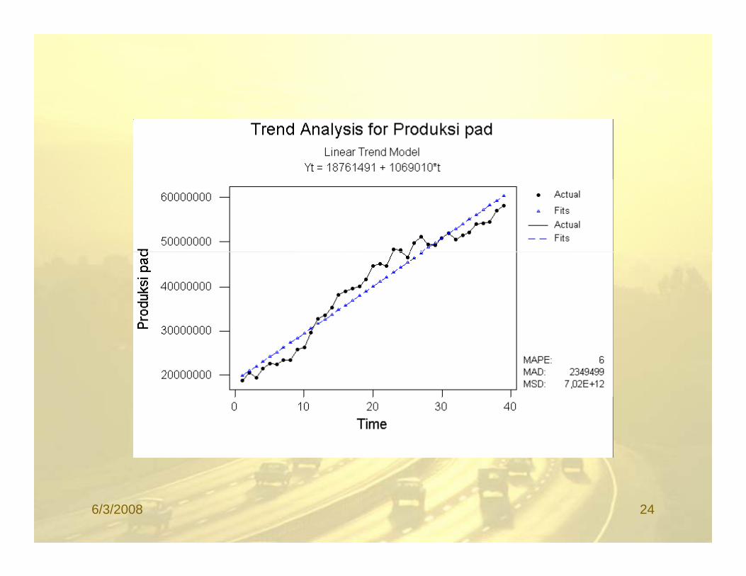
An Example• Hasil produksi padi Indonesia dari tahun 1970
sampai tahun 2008 sampai bulan Mei.• Hasil produksi ini berdasarkan musiman• Ada 39 tahun
6/3/2008 22

tahun produksi padi tahun produksi padi1970 18 693 649 1990 45 178 7511970 18.693.649 1990 45.178.751 1971 20.483.687 1991 44.688.247 1972 19.393.933 1992 48.240.009 1973 21.490.578 1993 48.181.087 1974 22.476.073 1994 46.641.524 1975 22.339.455 1995 49.744.140 1976 23.300.939 1996 51.101.506 1977 23.347.132 1997 49.377.054 1978 25.771.570 1998 49.236.692 1979 26.282.663 1999 50.866.387 1980 29.651.905 2000 51.898.852 1981 32 774 176 2001 50 460 7821981 32.774.176 2001 50.460.782 1982 33.583.677 2002 51.489.694 1983 35.303.106 2003 52.137.604 1984 38.136.446 2004 54.088.468 1985 39 032 945 2005 54 151 0971985 39.032.945 2005 54.151.097 1986 39.726.761 2006 54.454.937 1987 40.078.195 2007 57.051.679 1988 41.676.170 2008 58.268.796 1989 44.725.582
6/3/2008 23
6/3/2008 24

Moving Averages
$YY Y Yt t-1 t- +1k=
+ +1Yt k+1
No general method exists for determining k.
We must try out several k values to see what works best.
6/3/2008 25

Implementing the Model
6/3/2008 26
A Comment on Comparing MSE Values
• Care should be taken when comparing MSE values of two different forecasting techniquesvalues of two different forecasting techniques.
• The lowest MSE may result from a technique that fits older values very well but fits recent valuesfits older values very well but fits recent values poorly.
• It is sometimes wise to compute the MSE using only the most recent values.
6/3/2008 27

Forecasting With The Moving Average Model
Forecasts for time periods 25 and 26 at time period 24:
$YY Y 36 + 3524 23 355
+
Forecasts for time periods 25 and 26 at time period 24:
.Y2 225 355= = =
$$Y Y 35 5 + 36+$ .YY Y
235.5 + 36
22625 24 35 75=+
= =
6/3/2008 28
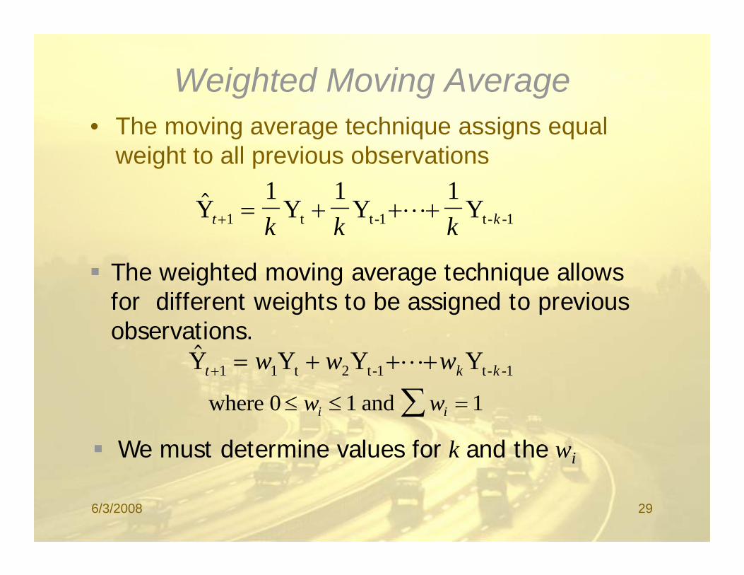
Weighted Moving Average• The moving average technique assigns equal
weight to all previous observations
$Y1
Y1
Y1
Yt t-1 t- -1t kk k k+ = + + +1 L
The weighted moving average technique allows for different weights to be assigned to previous b tiobservations.
$Y Y Y Yt t-1 t- -1t k kw w w+ = + + +1 1 2 L
h 0 d≤ ≤ ∑1 1where 0 and ≤ ≤ =∑w wi i1 1
We must determine values for k and the wi
6/3/2008 29
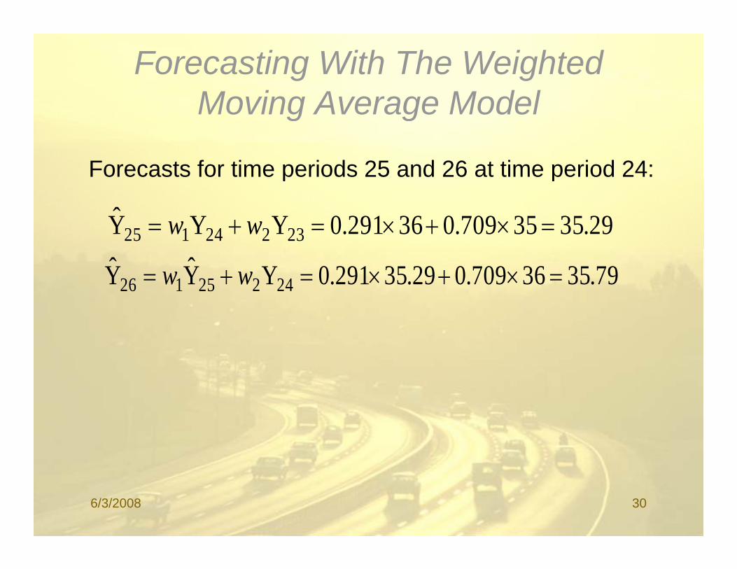
Forecasting With The Weighted Moving Average ModelMoving Average Model
Forecasts for time periods 25 and 26 at time period 24:
29.3535709.036291.0YYY 23224125 =×+×=+= ww
p 5 6 p
79.3536709.029.35291.0YYY 24225126 =×+×=+= ww
6/3/2008 30
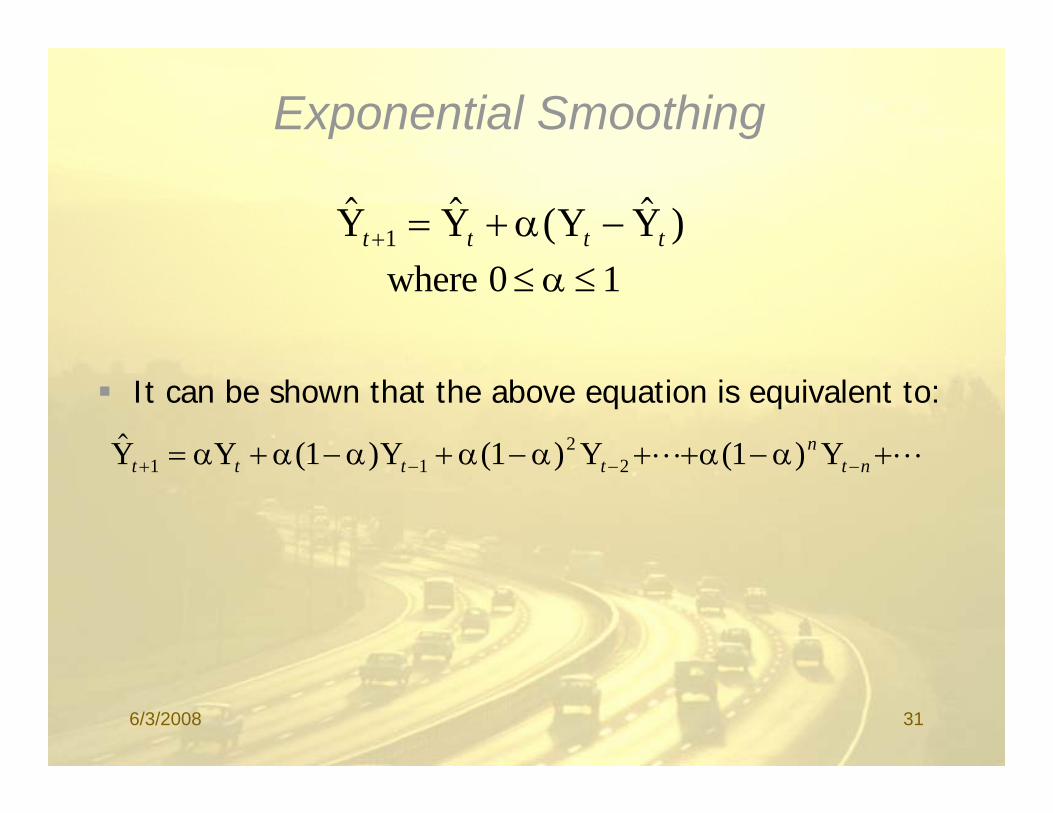
Exponential Smoothing
$ $ ( $ )Y Y Y Yt t t t+ = + −1 αwhere 0 1≤ ≤α
It can be shown that the above equation is equivalent to:
$ ( ) ( ) ( )Y Y Y Y Yn= + − + − + + − +21 1 1α α α α α α αL L( ) ( ) ( )Y Y Y Y Yt t t t t n+ − − −= + + + + +1 1 21 1 1α α α α α α α
6/3/2008 31

Examples of TwoExponential Smoothing Functions
42
38
40
34
36
nits
Sol
d
32
34
Un
Number of VCRs Sold
28
30
1 2 3 4 5 6 7 8 9 10 11 12 13 14 15 16 17 18 19 20 21 22 23 24 25
Exp. Smoothing alpha=0.1Exp. Smoothing alpha=0.9
Time Period6/3/2008 32
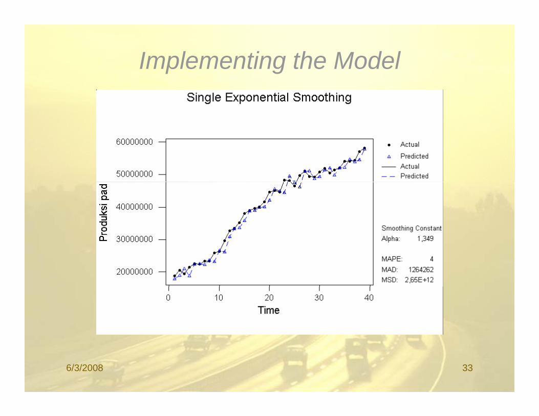
Implementing the Model
6/3/2008 33
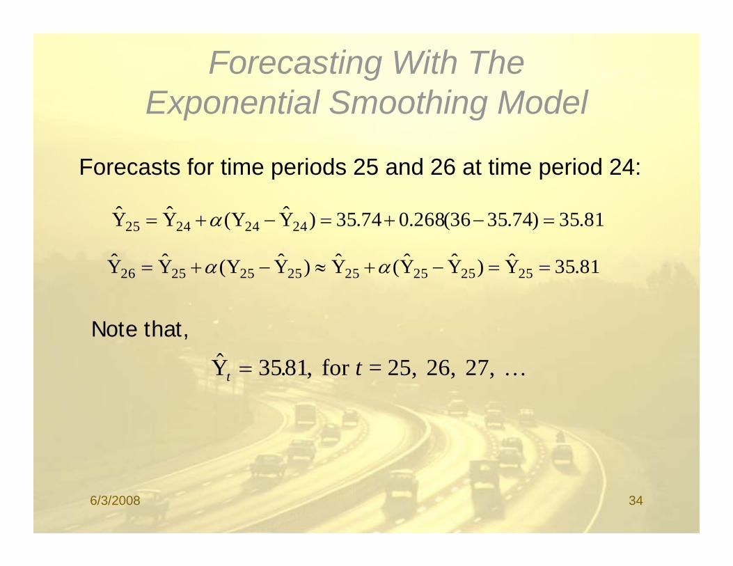
Forecasting With The Exponential Smoothing ModelExponential Smoothing Model
Forecasts for time periods 25 and 26 at time period 24:
81.35)74.3536(268.074.35)YY(YY 24242425 =−+=−+= α
p p
81.35Y)YY(Y)YY(YY 2525252525252526 ==−+≈−+= αα
$ . ,Y for = 25, 26, 27, t t= 3581 K
Note that,
6/3/2008 34

6/3/2008 35

Seasonality
• Seasonality is a regular, repeating pattern in time series data.
• May be additive or multiplicative in y pnature...
6/3/2008 36
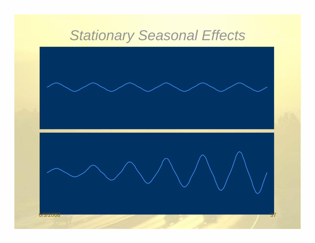
Stationary Seasonal EffectsAdditive Seasonal Effects
1 2 3 4 5 6 7 8 9 10 11 12 13 14 15 16 17 18 19 20 21 22 23 24 25
Tim e Pe r iod
Multiplicative Seasonal Effects
1 2 3 4 5 6 7 8 9 10 11 12 13 14 15 16 17 18 19 20 21 22 23 24 25
Tim e Pe r iod
6/3/2008 37
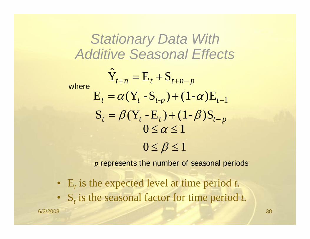
Stationary Data With yAdditive Seasonal Effects
+SEY pnttnt −++ += SEYwhere
1)E-(1)S-Y(E −+= tt-ptt αα
ptttt −+= )S-(1)E-Y(S ββ10 ≤≤α10 ≤≤ β
p represents the number of seasonal periodsp represents the number of seasonal periods
• Et is the expected level at time period t.S i th l f t f ti i d t• St is the seasonal factor for time period t.
6/3/2008 38

Implementing the Model
6/3/2008 39

Forecasting With The AdditiveSeasonal Effects ModelSeasonal Effects Model
Forecasts for time periods 25 to 28 at time period 24:p p
4242424 SEY −++ += nn
00.36345.844.354SEY 212425 =+=+=
73336821744354SEY 73.33682.1744.354SEY 222426 =−=+=
13401584644354SEY 232427 =+=+= 13.40158.4644.354SEY 232427 ++
81.32273.3144.354SEY 242428 =−=+=
6/3/2008 40

Stationary Data With yMultiplicative Seasonal Effects
Sˆpnttnt −++ ×= SEY
where
1)E-(1)/SY(E −+= tt-ptt αα 1)()( tt ptt
ptttt −+= )S-(1)/EY(S ββ10 ≤≤α1010
≤≤≤≤
βα
p represents the number of seasonal periodsp represents the number of seasonal periods
• Et is the expected level at time period t.• St is the seasonal factor for time period t.
6/3/2008 41

Forecasting With The MultiplicativeSeasonal Effects ModelSeasonal Effects Model
Forecasts for time periods 25 to 28 at time period 24:
4242424 SEY −++ ×= nn
13.359015.195.353SEY 212425 =×=×=ˆ 94.334946.044.354SEY 222426 =×=×=
99400133144354SEY =×=×= 99.400133.144.354SEY 232427 =×=×=
95.322912.044.354SEY 242428 =×=×=
6/3/2008 42
Trend Models
• Trend is the long-term sweep or general direction of movement in a time series.
• We’ll now consider some nonstationary time series techniques that are appropriate for data exhibiting upward or downward trends.
6/3/2008 43

An Examplep• WaterCraft Inc. is a manufacturer of personal
water crafts (also known as jet skis)water crafts (also known as jet skis). • The company has enjoyed a fairly steady
growth in sales of its productsgrowth in sales of its products.• The officers of the company are preparing sales
and manufacturing plans for the coming year. a d a u actu g p a s o t e co g yea• Forecasts are needed of the level of sales that
the company expects to achieve each quarter. p y p q• See file
6/3/2008 44
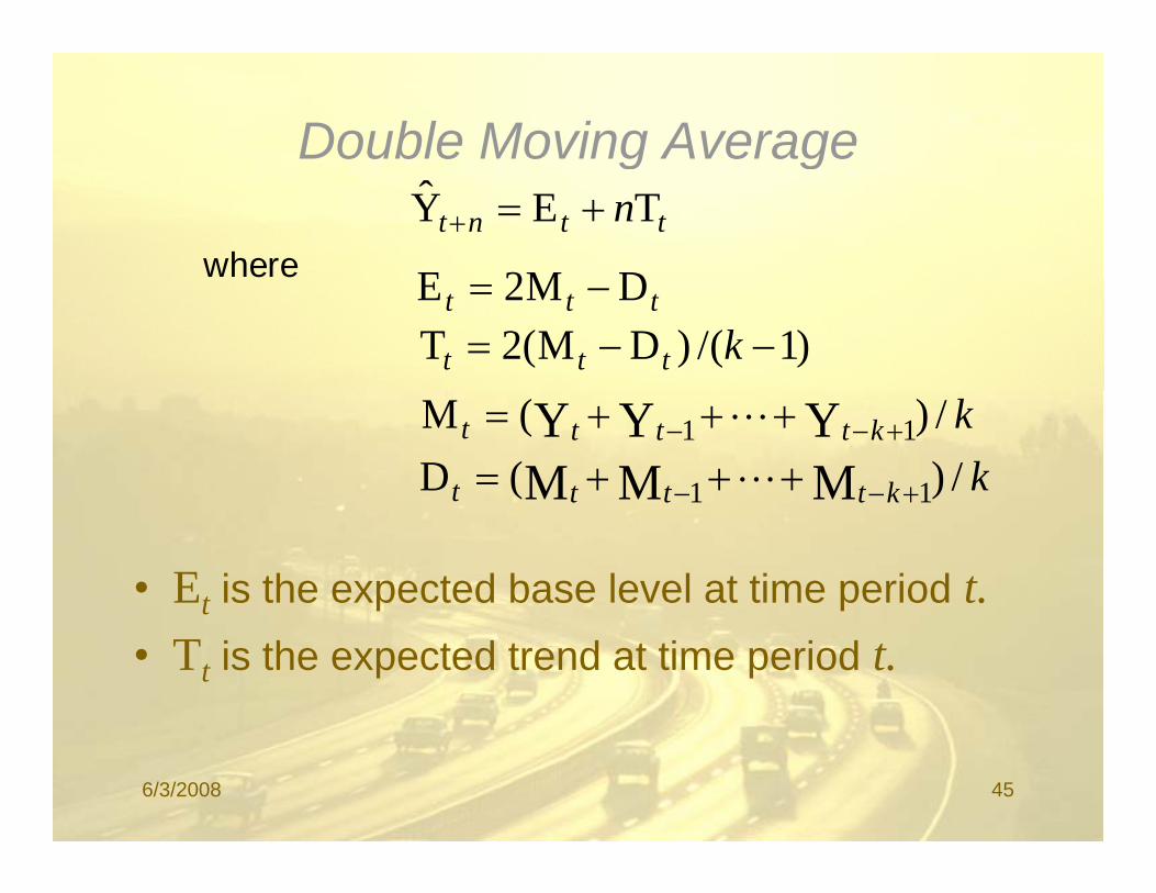
Double Moving Averageg gttnt nTEY +=+
where DM2E ttt DM2E −=)1/()DM(2T −−= kttt
kktttt /)(M YYY 11 +−− +++= L
kktttt /)(D MMM 11 +−− +++= L
• Et is the expected base level at time period t.• Tt is the expected trend at time period t.
6/3/2008 45
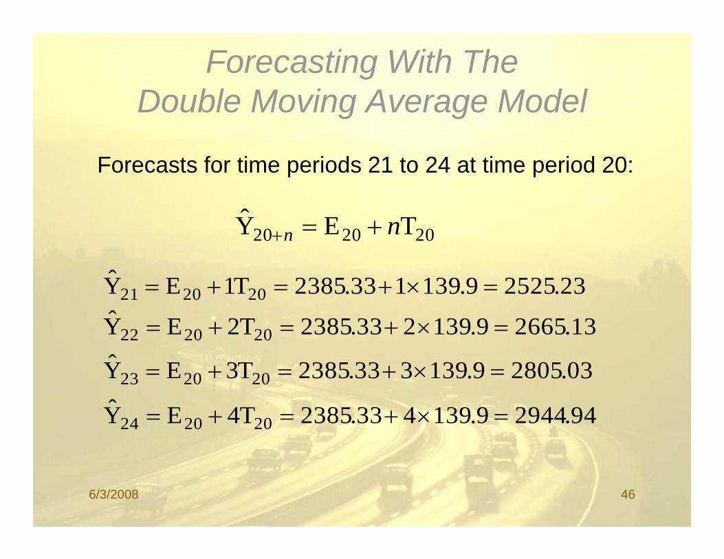
Forecasting With The Double Moving Average ModelDouble Moving Average Model
Forecasts for time periods 21 to 24 at time period 20:p p
202020 TEY nn +=+
23.25259.139133.2385T1EY 202021 =×+=+=ˆ 13.26659.139233.2385T2EY 202022 =×+=+=
03.28059.139333.2385T3EY 202023 =×+=+=
94.29449.139433.2385T4EY 202024 =×+=+=
6/3/2008 46

Double Exponential Smoothing(Holt’s Method)(Holt s Method)
TEY + ttnt nTEY +=+
whereEt = αYt + (1-α)(Et-1+ Tt-1)Tt = β(Et −Et-1) + (1-β) Tt-1
• E is the expected base level at time period t
0 1 1≤ ≤ ≤ ≤α βand 0
• Et is the expected base level at time period t.• Tt is the expected trend at time period t.
6/3/2008 47
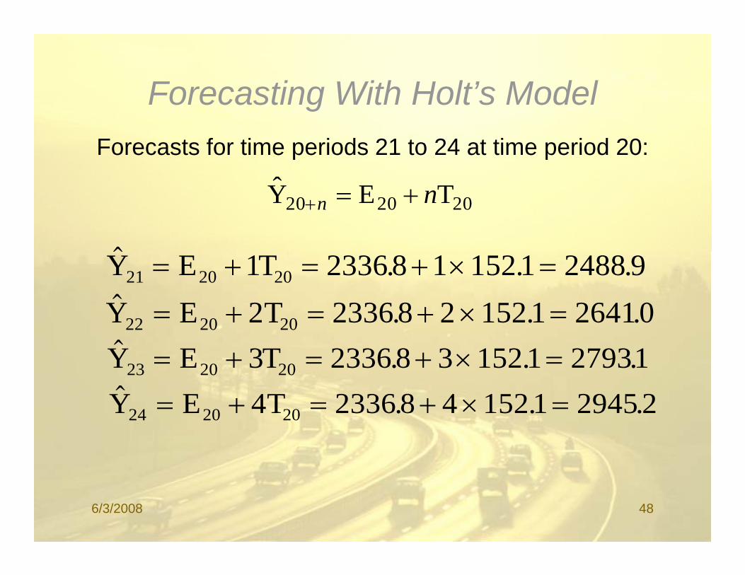
Forecasting With Holt’s ModelgForecasts for time periods 21 to 24 at time period 20:
ˆ
$
202020 TEY nn +=+
$ . . .Y E T21 20 201 2336 8 1 152 1 2488 9= + = + × =$ . . .Y E T22 20 202 2336 8 2 152 1 26410= + = + × =22 20 20
$ . . .Y E T23 20 203 2336 8 3 152 1 27931= + = + × =$Y E T4 2336 8 4 152 1 2945 2. . .Y E T24 20 204 2336 8 4 152 1 2945 2= + = + × =
6/3/2008 48

Holt-Winter’s Method For Additive Seasonal Effects
n ++= STEY pntttnt n −++ ++= STEYwhere
( ) )T)(E(1SYE ++ αα( ) )T)(E-(1SYE 11 −−− ++−= ttpttt αα( ) 11 )T-(1EET −− +−= tttt ββ( ) ptttt −+−= )S-(1EYS γγ
10 ≤≤α
101010
≤≤≤≤
βα
10 ≤≤ γ6/3/2008 49
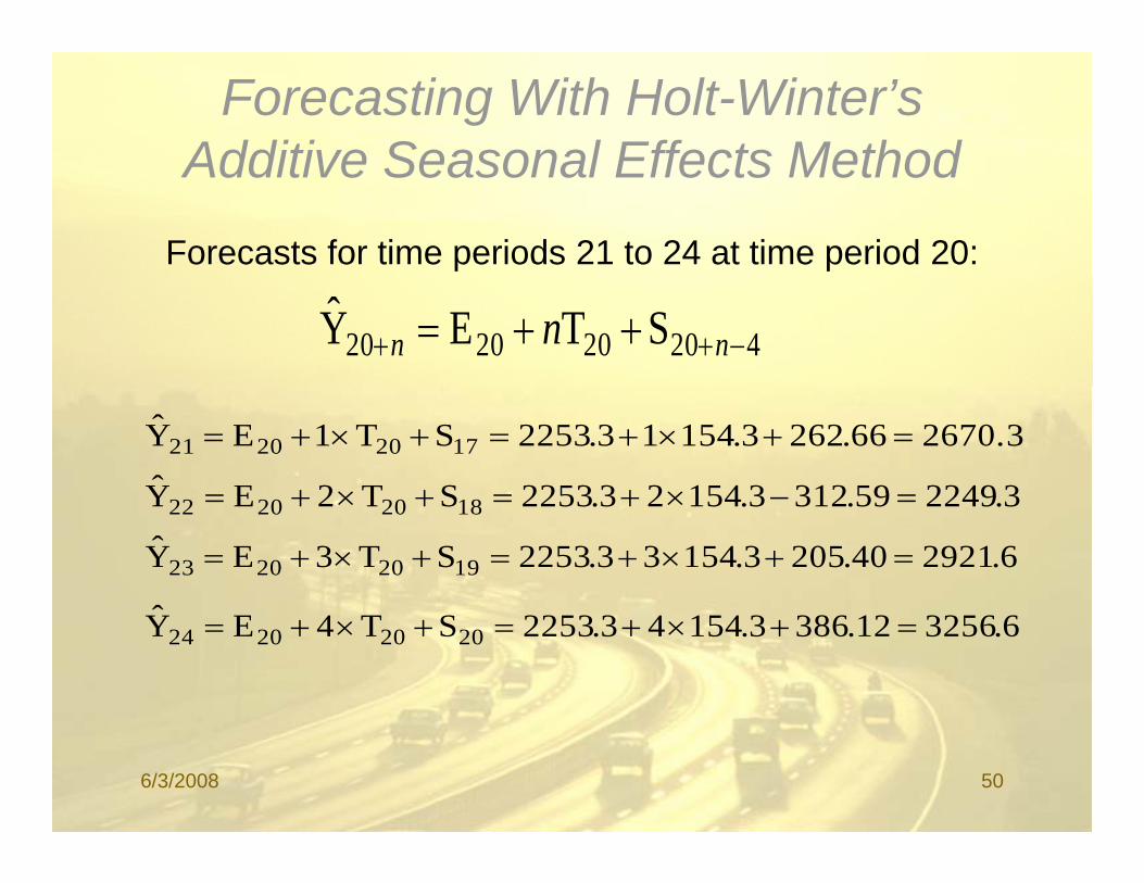
Forecasting With Holt-Winter’s Additive Seasonal Effects MethodAdditive Seasonal Effects Method
Forecasts for time periods 21 to 24 at time period 20:
420202020 STEY −++ ++= nn n
2670.366.2623.15413.2253ST1EY 17202021 =+×+=+×+=
32249593123154232253ST2EY =−×+=+×+= 3.224959.3123.15423.2253ST2EY 18202022 =−×+=+×+=
6.292140.2053.15433.2253ST3EY 19202023 =+×+=+×+=
ˆ 6.325612.3863.15443.2253ST4EY 20202024 =+×+=+×+=
6/3/2008 50
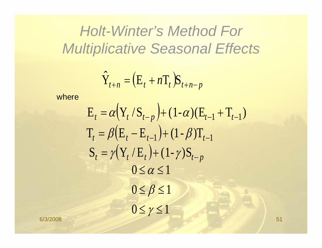
Holt-Winter’s Method For M ltiplicati e Seasonal EffectsMultiplicative Seasonal Effects
( )STEY ( ) pntttnt n −++ += STEYwhere
( ) )T)(E(1S/YE ( ) )T)(E-(1S/YE 11 −−− ++= ttpttt αα( ) 11 )T-(1EET −− +−= tttt ββ ( ) 11 )( tttt ββ( ) ptttt −+= )S-(1E/YS γγ
10 ≤≤α1010
≤≤≤≤
βα
10 ≤≤ γ6/3/2008 51

Forecasting With Holt-Winter’s Multiplicative Seasonal Effects MethodMultiplicative Seasonal Effects Method
Forecasts for time periods 21 to 24 at time period 20:p p
( ) 420202020 S TEY −++ += nn n
7.2713152.1)3.13716.2217()T1E(Y 17202021 =×+=+= S
ˆ 9.2114849.0)3.13726.2217()T2E(Y 18202022 =×+=+= S
5.2900103.1)3.13736.2217()T3E(Y 19202023 =×+=+= S )()( 19202023
9.3293190.1)3.13746.2217()T4E(Y 20202024 =×+=+= S
6/3/2008 52

The Linear Trend Model
$Y Xb b= +Y Xt b bt
= +0 1 1
t=1Xwhere tt1X where
For example:For example:
X X X 1 1 11 2 31 2 3= = =, , , K
6/3/2008 53

Forecasting With Th Li T d M d lThe Linear Trend Model
Forecasts for time periods 21 to 24 at time period 20:
$ . . .Y X21 0 1 1213751 92 6255 21 2320 3= + = + × =b b
$ . . .Y X22 0 1 1223751 92 6255 22 2412 9= + = + × =b b
$Y X 3751 92 6255 23 25056= + = + × =b b . . .Y X23 0 1 1233751 92 6255 23 25056= + = + × =b b
$ . . .Y X24 0 1 1243751 92 6255 24 2598 2= + = + × =b b
6/3/2008 54

The TREND() FunctionTREND(Y-range, X-range, X-value for prediction)
where: Y range is the spreadsheet range containing the dependentY-range is the spreadsheet range containing the dependent Y variable, X-range is the spreadsheet range containing the independent X variable(s), X-value for prediction is a cell (or cells) containing the values for the independent X variable(s) for which we want p ( )an estimated value of Y.
Note: The TREND( ) function is dynamically updated wheneverNote: The TREND( ) function is dynamically updated whenever any inputs to the function change. However, it does not provide the statistical information provided by the regression tool. It is best two use these two different approaches to doing regressionbest two use these two different approaches to doing regression in conjunction with one another. 6/3/2008 55
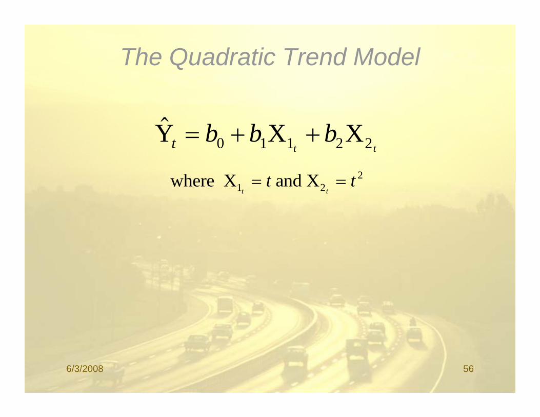
The Quadratic Trend Model
$Y X Xb b b+ +Y X Xt b b bt t
= + +0 1 1 2 2
where X and X 2t t= =where X and X1 2t tt t= =
6/3/2008 56

Forecasting With The Quadratic Trend Model
Forecasts for time periods 21 to 24 at time period 20:
9.259821617.321671.1667.653XXY 22211021 2121
=×+×+=++= bbb
12771226173226711667653XXY 2bbb 1.277122617.322671.1667.653XXY 22211022 2222
=×+×+=++= bbb
4.295023617.323671.1667.653XXY 22211023 2323
=×+×+=++= bbb
1.313724617.324671.1667.653XXY 22211024 2424
=×+×+=++= bbb
6/3/2008 57
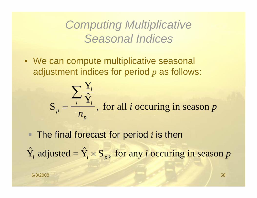
Computing Multiplicative Seasonal IndicesSeasonal Indices
• We can compute multiplicative seasonal• We can compute multiplicative seasonal adjustment indices for period p as follows:
Y∑S
YY
, for all occuring in season p
i
ii i p=∑ $
gppn
p
The final forecast for period i is thenThe final forecast for period i is then
$ $Y adjusted = Y S , for any occuring in season i i p i p×
6/3/2008 58

Forecasting With Seasonal Factors Applied To The Quadratic Trend ModelApplied To The Quadratic Trend Model
Forecasts for time periods 21 to 24 at time period 20:Forecasts for time periods 21 to 24 at time period 20:
8.2747%7.1059.2598)XX(Y 12211021 2121=×=++= Sbbb
6.2219%1.801.2771)XX(Y 22211022 2222=×=++= Sbbb
43041%110352950)XX(Y ++ Sbbb 4.3041%1.1035.2950)XX(Y 32211023 2323=×=++= Sbbb
1.3486%1.1112.3137)XX(Y 42211024 2424=×=++= Sbbb
6/3/2008 59
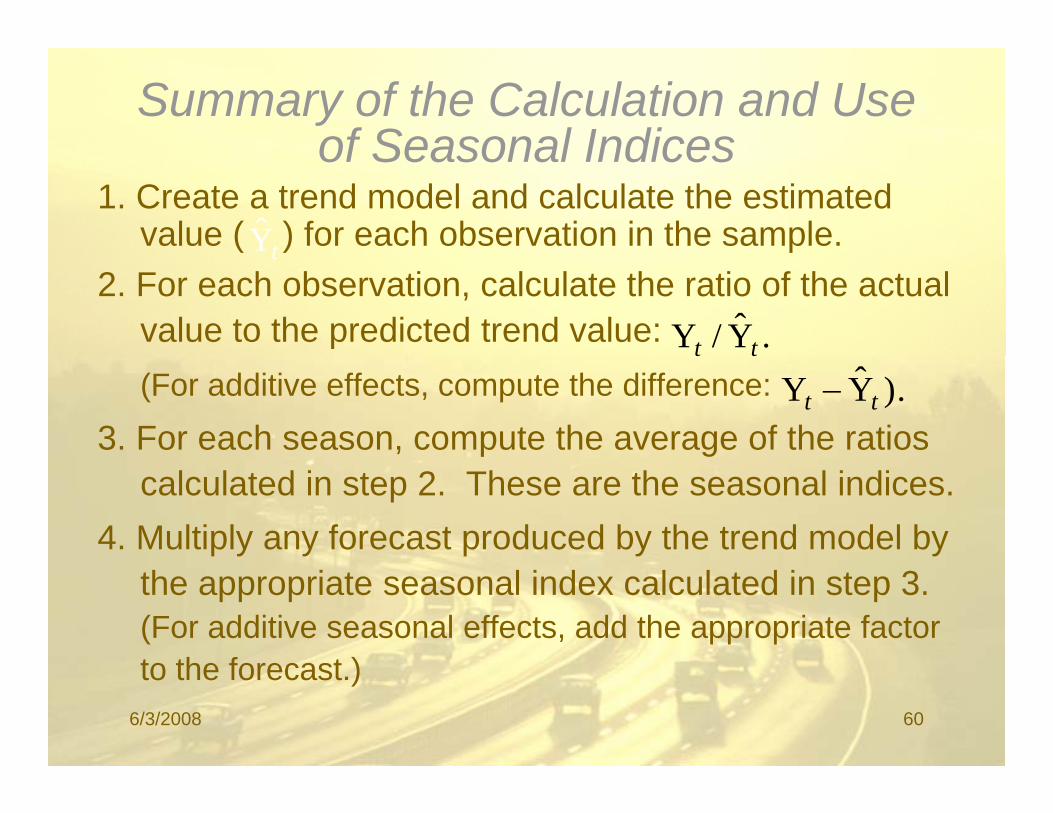
Summary of the Calculation and Use of Seasonal Indicesof Seasonal Indices
1. Create a trend model and calculate the estimated value ( ) for each observation in the sample.tY( )
2. For each observation, calculate the ratio of the actual value to the predicted trend value:
t
.Y/Y tt(For additive effects, compute the difference:
3. For each season, compute the average of the ratios
tt
).YY tt −
calculated in step 2. These are the seasonal indices.4. Multiply any forecast produced by the trend model by
the appropriate seasonal index calculated in step 3. (For additive seasonal effects, add the appropriate factor to the forecast )to the forecast.)
6/3/2008 60

Refining the Seasonal Indicese g t e Seaso a d ces• Note that Solver can be used to simultaneously
determine the optimal values of the seasonaldetermine the optimal values of the seasonal indices and the parameters of the trend model being used.being used.
• There is no guarantee that this will produce a better forecast, but it should produce a model , pthat fits the data better in terms of the MSE.
See file Fig11-39.xls
6/3/2008 61
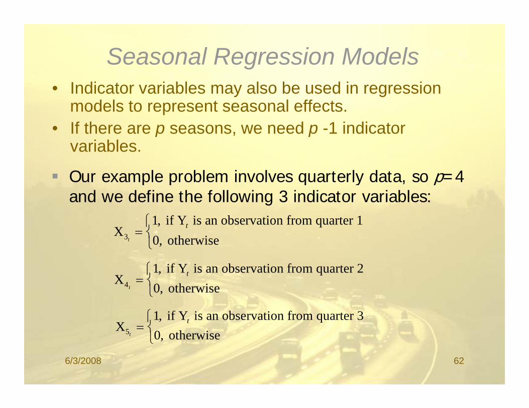
Seasonal Regression Models• Indicator variables may also be used in regression
models to represent seasonal effects.• If there are p seasons we need p 1 indicator• If there are p seasons, we need p -1 indicator
variables.
Our example problem involves quarterly data so p=4Our example problem involves quarterly data, so p=4 and we define the following 3 indicator variables:
X if Y is an observation from quarter 11 t⎧
⎨,
X if Y is an observation from quarter 21 t=
⎧⎨
,
X otherwise3 0t
= ⎨⎩ ,
Xotherwise4 0t
= ⎨⎩ ,
X if Y is an observation from quarter 3
th i5
10
t=⎧⎨⎩
,otherwise5 0t
⎨⎩ ,
6/3/2008 62
Implementing the Model
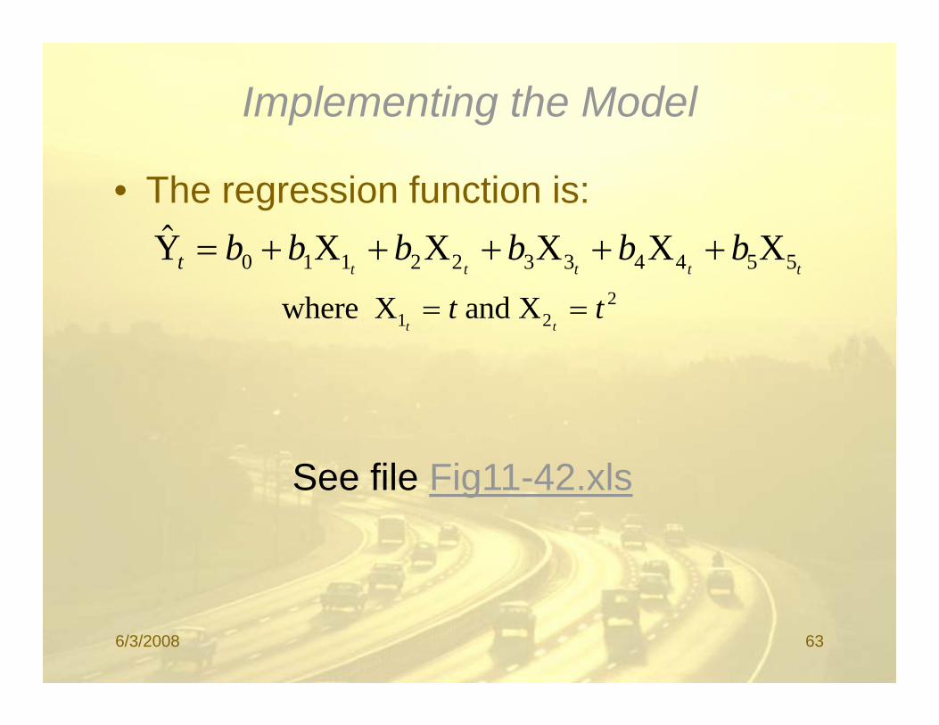
• The regression function is:$$Y X X X X Xt b b b b b b
t t t t t= + + + + +0 1 1 2 2 3 3 4 4 5 5
where X and X1 22t t= =where X and X1 2t t
t t
See file Fig11-42.xls
6/3/2008 63

Forecasting With The S l R i M d lSeasonal Regression Model
Forecasts for time periods 21 to 24 at time period 20:
5.2638)0(453.123)0(736.424)1(805.86)21(485.3)21(319.17471.824Y 221 =−−−++=
ˆ 2 7.2467)0(453.123)1(736.424)0(805.86)22(485.3)22(319.17471.824Y 222 =−−−++=
2.2943)1(453.123)0(736.424)0(805.86)23(485.3)23(319.17471.824Y 223 =−−−++=
8.3247)0(453.123)0(736.424)0(805.86)24(485.3)24(319.17471.824Y 224 =−−−++=
6/3/2008 64

StatTools
• StatTools is an add-in that simplifies theStatTools is an add in that simplifies the process of performing time series analysis in Excel.
• A trial version of StatTools is available on the CD-ROM accompanying this book.p y g
• For more information on StatTools see:http://www.palisade.comhttp://www.palisade.com
6/3/2008 65
Combining Forecasts
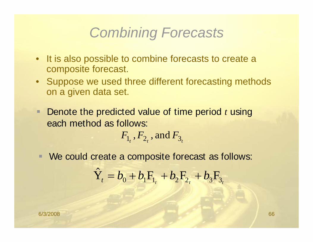
• It is also possible to combine forecasts to create a composite forecast.
• Suppose we used three different forecasting methods on a given data set.
Denote the predicted value of time period t using each method as follows:
FFF 321 andttt
FFF 321 and,,
We could create a composite forecast as follows:
$Y F F Ft b b b bt t t
= + + +0 1 1 2 2 3 3
6/3/2008 66

ARIMA Model: Produksi padi
ARIMA model for Produksi padiARIMA model for Produksi padi
Estimates at each iterationIteration SSE Parameters
0 451374984309793 0,100 0,100 0,100 0,1001 368364447306473 0,021 0,199 0,250 0,1522 325456920491419 -0,129 0,154 0,348 0,1863 285571989081979 -0,279 0,118 0,475 0,2294 245711224167492 -0,324 0,193 0,542 0,1875 187899115792845 -0,474 0,260 0,657 0,0416 155112700780088 -0,527 0,353 0,704 -0,1097 141714161123773 0 447 0 503 0 647 0 2017 141714161123773 -0,447 0,503 0,647 -0,2018 129630495049884 -0,368 0,653 0,585 -0,2879 117486920579732 -0,301 0,803 0,523 -0,376
10 101549593049237 -0,291 0,953 0,498 -0,50311 87502739697009 -0,393 1,051 0,567 -0,65312 81737678770148 -0,543 1,076 0,614 -0,708, , , ,13 79314052359269 -0,619 1,074 0,596 -0,68714 79233477547537 -0,622 1,073 0,587 -0,67715 79162421478230 -0,620 1,072 0,581 -0,67116 79124151604006 -0,619 1,071 0,577 -0,66717 79104368397552 -0,619 1,071 0,576 -0,66518 79092164140468 -0,619 1,070 0,575 -0,66419 79085747120700 -0,620 1,070 0,575 -0,664
Relative change in each estimate less than 0,0010
6/3/2008 67

Final Estimates of ParametersType Coef SE Coef T PType Coef SE Coef T PAR 1 -0,6197 0,1611 -3,85 0,001MA 1 1,0698 0,0298 35,85 0,000MA 2 0,5753 0,1894 3,04 0,005MA 3 -0,6641 0,1882 -3,53 0,001MA 3 0,6641 0,1882 3,53 0,001
Differencing: 3 regular differencesNumber of observations: Original series 39, after differencing 36Residuals: SS = 70758139198041 (backforecasts excluded)es dua s SS 0 58 39 980 (bac o ecasts e c uded)
MS = 2211191849939 DF = 32
Modified Box-Pierce (Ljung-Box) Chi-Square statisticLag 12 24 36 48gChi-Square 20,9 38,4 * *DF 8 20 * *P-Value 0,008 0,008 * *
6/3/2008 68

Model-model Time Series Regressiong
1. Model Regresi untuk LINEAR TRENDYt = a + b.t + error t = 1, 2, … (dummy waktu)
2. Model Regresi untuk Data SEASONAL (variasi konstan)Yt = a + b1 D1 + … + bS-1 DS-1 + error
dengan : D1 D2 DS 1 adalah dummy waktu dalamdengan : D1, D2, …, DS-1 adalah dummy waktu dalam satu periode seasonal.
3. Model Regresi untuk Data dengan LINEAR TREND dan SEASONAL (variasi konstan)
Yt = a + b.t + c1 D1 + … + cS-1 DS-1 + errorGabungan model 1 dan 2.
6/3/2008 69

Naïve ModelNaïve Model
The recent periods are the best predictors of the future.
1. The simplest model for stationary data isˆ
2. The simplest model for trend data is
tt YY =+1
)(ˆ YYYY or
11
ˆ−
+ =t
ttt Y
YYY
)( 11 −+ −+= tttt YYYY
3. The simplest model for seasonal data is
stt YY −++ = )1(1ˆ
6/3/2008 70

Average MethodsAverage Methods
1. Simple Averagesobtained by finding the mean for all the relevant values and then using this mean to forecast the next period.g p
∑=
+ =n
t
tt n
YY1
1ˆ for stationary data
2. Moving Averagesobtained by finding the mean for a specified set of valuesand then using this mean to forecast the next periodand then using this mean to forecast the next period.
nYYYYM nttt
tt)(ˆ 11
1+−−
++++
==K
for stationary data
6/3/2008 71

Average Methods … (continued)Average Methods … (continued)
3. Double Moving Averagesone set of moving averages is computed, and then a second set is computed as a moving average of the first set.
(i).
(ii)
nYYYYM nttt
tt)(ˆ 11
1+−−
++++
==K
MMM nttt )( 11 ++++′ K(ii).
(iii).
nMMMM nttt
t)( 11 +−− +++
=′K
ttt MMa ′−= 2
(iv).
pbaY +ˆ f li t d d t
)(1
2ttt MM
nb ′−
−=
pbaY ttpt +=+ for a linear trend data
6/3/2008 72
Exponential Smoothing MethodsExponential Smoothing Methods
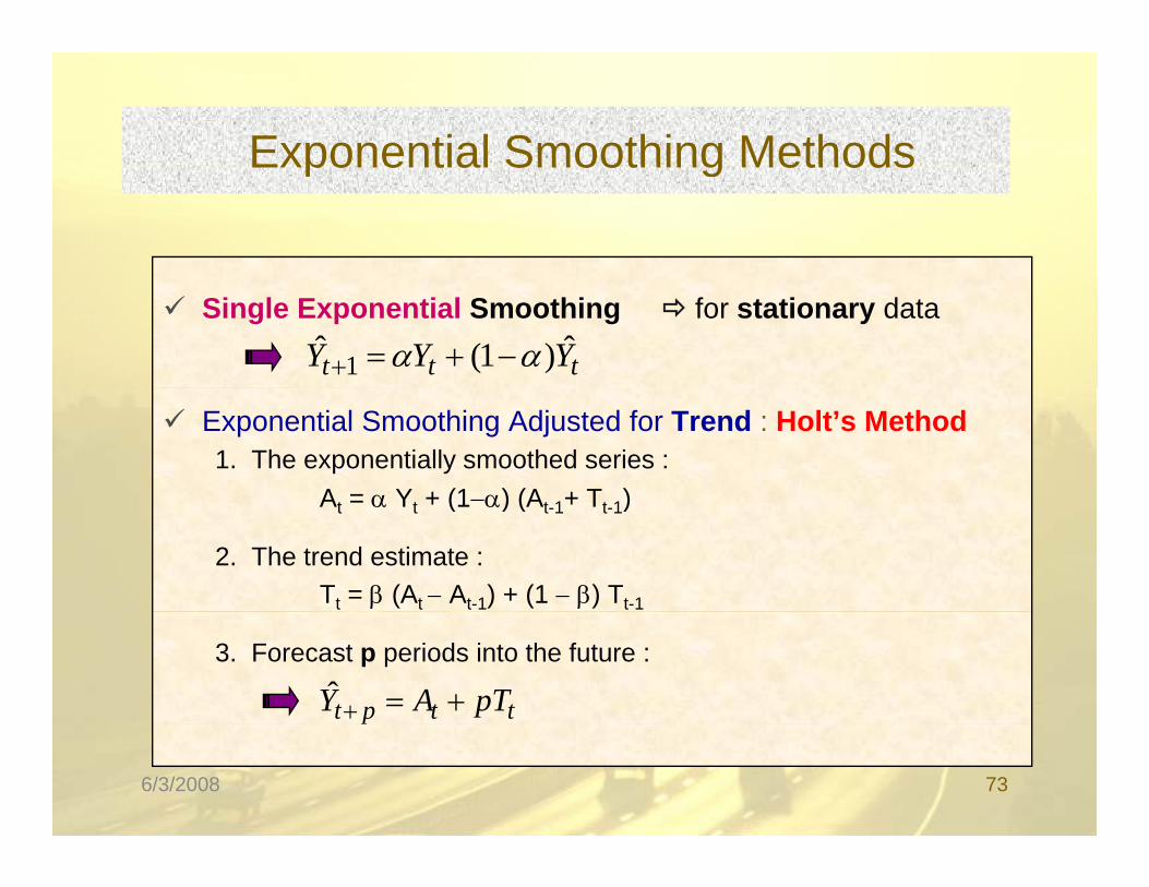
Single Exponential Smoothing for stationary data
ttt YYY ˆ)1(ˆ 1 αα −+=+
Exponential Smoothing Adjusted for Trend : Holt’s Method1. The exponentially smoothed series :
A = α Y + (1−α) (A + T )At = α Yt + (1−α) (At-1+ Tt-1)
2. The trend estimate :Tt = β (At − At-1) + (1 − β) Tt-1
3. Forecast p periods into the future :
ttpt pTAY +=+ˆ p
6/3/2008 73

Exponential Smoothing Adjusted for Trend and Seasonal Variation : Winter’s MethodSeasonal Variation : Winter’s Method
1. The exponentially smoothed series :
)( )1( 11 −−−
+−+= ttLt
tt TA
SYA αα
2. The trend estimate :
Lt
11 )1()( −− −+−= tttt TAAT ββThree
parameters
3. The seasonality estimate :
11 tttt
1)1( −+= tt
t SYS γγ
pmodels
4. Forecast p periods into the future :
1)1( −+ tt
t SA
S γγ
Ltttt SpTAY ++ −= )(ˆ pLtttpt SpTAY +−+ = )(
6/3/2008 74