Sains Malaysiana 44(12)(2015): 1721–1728

An Interactively Recurrent Functional Neural Fuzzy Network with Fuzzy Differential Evolution and Its Applications

(Rangkaian Neuron Kabur Berfungsi Interaktif Berulang dengan Evolusi Pengkamiran Kabur dan Penggunaannya)

CHENG-JIAN LIN*, CHIH-FENG WU, HSUEH-YI LIN & CHENG-YI YU

ABSTRACT

In this paper, an interactively recurrent functional neural fuzzy network (IRFNFN) with fuzzy differential evolution (FDE) learning method was proposed for solving the control and the prediction problems. The traditional differential evolution (DE) method easily gets trapped in a local optimum during the learning process, but the proposed fuzzy differential evolution algorithm can overcome this shortcoming. Through the information sharing of nodes in the interactive layer, the proposed IRFNFN can effectively reduce the number of required rule nodes and improve the overall performance of the network. Finally, the IRFNFN model and associated FDE learning algorithm were applied to the control system of the water bath temperature and the forecast of the sunspot number. The experimental results demonstrate the effectiveness of the proposed method.

Keywords: Control; differential evolution; neural fuzzy network; prediction; recurrent network

ABSTRAK

Dalam kajian ini, rangkaian neuron kabur berfungsi interaktif berulang (IRFNFN) dengan kaedah pembelajaran evolusi pengkamiran kabur (FDE) dicadangkan untuk menyelesaikan masalah kawalan dan ramalan. Kaedah tradisi evolusi pengkamiran (DE) akan terperangkap dengan mudah di dalam optimum tempatan semasa proses pembelajaran, tetapi evolusi pengkamiran kabur algoritma yang dicadangkan boleh mengatasi kelemahan ini. Melalui perkongsian maklumat nod dalam lapisan interaktif, IRFNFN yang dicadangkan boleh mengurangkan bilangan nod peraturan yang diperlukan dengan berkesan dan meningkatkan prestasi keseluruhan rangkaian. Akhir sekali, gabungan model IRFNFN dan pembelajaran algoritma FDE digunakan untuk sistem kawalan suhu rendaman air dan ramalan nombor tompok matahari. Keputusan eksperimen menunjukkan keberkesanan kaedah yang dicadangkan.

Kata kunci: Evolusi pengkamiran; kawalan; ramalan; rangkaian berulang; rangkaian neuron kabur

INTRODUCTION

In recent years, the applications of control theory to engineering system have been widely proposed. The engineering system in which the output data is not proportional to the input data, is called a nonlinear system. Controlling a nonlinear system is more difficult than controlling a linear one. Many researchers (Chen 2010; Juang & Hsieh 2010; Lee & Teng 2000; Lin et al. 2010) have conducted experiments to prove that the recurrent neural fuzzy network can achieve good results of the tracking, control and the prediction problems in complex nonlinear systems. The neural fuzzy networks commonly employ traditional learning methods, back propagation (BP) algorithm for example, to train the network parameters (Chen & Teng 1995; Li et al. 2012; Wang et al. 2011). However, BP algorithm is easily trapped into a local optimum solution. Many researchers (Chen et al. 2014; Juang 2002; Lin et al. 2009) introduced evolutionary optimization algorithms into the learning step of neural fuzzy network, and Genetic algorithm (GA) (Lin 2004) is one of the popular evolutionary algorithms. GA can explore the global

searching space efficiently, but the problems of the local optima trap and the premature convergence still exist. In 1995, the differential evolutionary (DE) algorithm was proposed by Storn and Price (1997). Due to its simple process, less parameters, high stability and powerful population-based stochastic search technique, the DE and modified DE algorithms get a good performance in some high-dimensional engineering problems (Neri & Tirronen 2010). The differential evolution algorithm is a kind of greedy method, which makes it converge quickly but gets trapped into the local optimum easily. Thus, Chen et al. (2009) combined the modified differential evolution algorithm in the parameter adjustment of the neural fuzzy network, Huang et al. (2006) provided some DE strategies to choose and self-adaptively control the parameters and Gong et al. (2011) presented a family of improved DEs that attempts to adaptively select a suitable strategy. In this paper, an interactively recurrent functional neural fuzzy network (IRFNFN) with fuzzy differential evolution (FDE) learning method was proposed for solving the control and the prediction problems. The proposed

1722

fuzzy differential evolution algorithm can improve the disadvantage of the local optimum trap in traditional DE. Moreover, the IRFNFN can effectively reduce the number of required rule nodes by sharing the information of the nodes in the interactive layer.

FUZZY DIFFERENTIAL EVOLUTION ALGORITHM

In order to achieve the adaptive searching, we use the diversities among the individuals as the inputs to the fuzzy membership functions, which inspire the corresponding strategies to adjust the parameters of DE.

FUZZY ADAPTIVE PARAMETER ADJUSTMENT

Improved differential evolution algorithm Compared to only one scale factor F in traditional DE/rand/1 method: (1)

and DE/current-to-best/1:

(2) We add an additional scale factor for more precisely controlling the convergence speed and the direction of flight.

(3) The denotes the individual i in the population, where i=1, 2,…, NP, and NP is the total number of the population. G denotes the generation and r1, r2 and r3 ∈ (1, NP) are random integers but r1 ≠ r2 ≠ r3 ≠ i. This new method improves the DE not easily to converge prematurely. Moreover, since there was no tractive phenomenon between these two scale factors, the new mutation method would not be trapped into a local optimum while this algorithm converging.

ASSESSMENT OF EVOLUTION STATUS

Evolutionary status is a measurement of diversity among the individuals distributed in the searching space. In each generation, a status factor f is produced, and then this algorithm adjusts the parameters F and CR in DE algorithm based on the status factor f. In order to obtain the status factor f, the individual diversities were calculated first.

(4)

where N and D represent the number of individuals with the dimension D and di is the difference degree between current individual and others. Then, the state factor was calculated as:

f = (dg – dmin)/(dmax – dmin), (5)

where dg represents the diversity of the current optimum solution and dmin and dmax represent the minimum and the maximum values among all diversities. In addition, to increase the effect of disturbance on DE, we added a random selection scheme, which provides an equal probability, 1/NP, to randomly select an individual diversity as dg. Then, it makes the proposed method not to use the same strategy persistently.

FUZZY STRATEGY

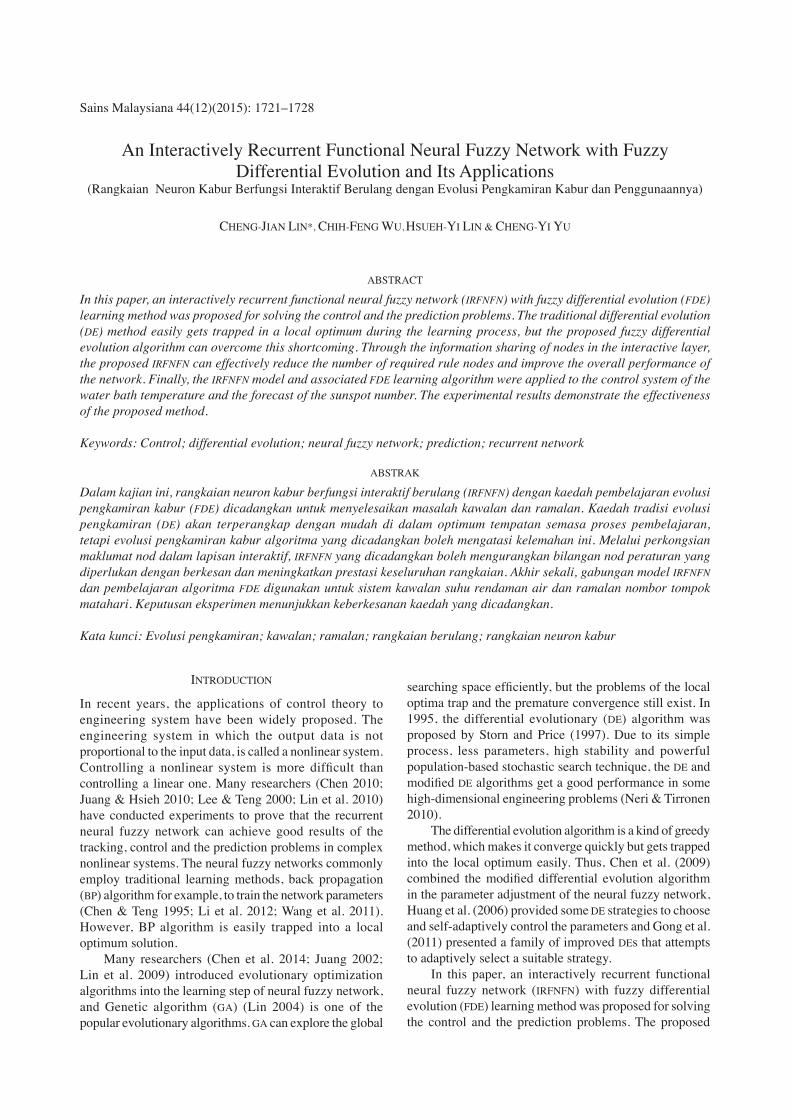
We took the status factor as the input of fuzzy membership function, and it inspires the strategies, S1, S2, S3 and S4, through the fuzzy inference. The followings are the fuzzy membership functions, as illustrated in Figure 1.

(6)

(7)

(8)

(9)

PARAMETERS ADJUSTMENT

F and CR are important parameters in DE, where CR is the crossover rate and CR ∈ [0,1]. Most articles set CR=0.9 for better use (Saruhan 2014; Simon 2013; Yang et al. 2010) and on most real world problems, Cr = 0.9 has become the standard, which works well across a large range of problem domains (Montgomery et al. 2010). In this study, we adjusted F1, F2 and CR adaptively according to f. The CR is adjusted through the following simple equation:

CR = 0.1 * f + 0.9. (10)

Then, we use the adaptive strategy inspired by fuzzy reasoning to adjust F1 and F2. The activation of strategy 1 is regarded as a regional search, thus we increase the value of F1 significantly to enlarge disturbances. When strategy 2 was used, we increase F2 significantly to make

1723

the individual move in the direction toward the current global solution. All the strategies are tabulated in Table 1.

GAUSSIAN DISTURBANCE

The rapid convergence of hyper-heuristic algorithm usually makes the algorithm get trapped in a local optimum. Therefore, many researchers incorporated the Gaussian disturbance method in these algorithms (Natsuki & Hitoshi 2003). The original Gaussian disturbance used a fixed constant σ. But in this study, we reform a linearly decreased σ to increase the adaptability

mut(x) = x * ( 1 + gaussian(σ)) (11)

σ = 1.0 – (1.0 – 0.1) * (g/G), (12)

where g and G represent the numbers of the current generation and the total generation of evolution. When the current generation of the evolutionary process is getting closer to end, the occurrence probability is getting lower and near 0.1.

EXPERIMENTAL DETAILS

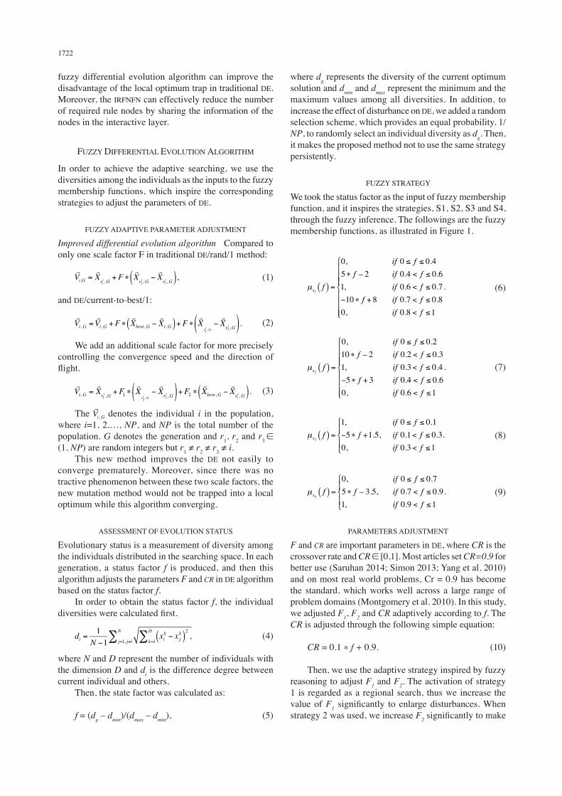
The performance of FDE was compared with DE/rand/1(DE) and DE/current-to-best/1(DEbest) on five well-known benchmark functions (Ali et al. 2005; Shang & Qin 2006), listed in Table 2. Among them, f1-f4 is single peak optimization problems, and f5 is multimodal problems. In our experiment, the dimension was set to 30 and the number of individuals was set to 100. The simulation results are tabulated in Table 3 and the results showed that the performance of the proposed FDE algorithm can exceed the performances of other DE algorithms.

AN INTERACTIVELY RECURRENT FUNCTIONAL NEURAL FUZZY NETWORK

In this section, we describe the structure of interactively recurrent functional neural fuzzy network (IRFNFN). The IRFNFN model adopts the interactive layer between the fuzzy-rule layer and the consequent layer in the recurrent functional neural fuzzy network (RFNFN). Through the

FIGURE 1. Fuzzy membership functions

TABLE 1. Strategies of fuzzy differential evolution

F1 F2

strategy 1strategy 2strategy 3strategy 4

large increasesmall increasesmall decreaselarge decrease

small increaselarge increaselarge decreasesmall decrease

TABLE 2. Benchmark functions

Test functions S

[-100,100]D

[-10,10]D

[-100,100]D

[-100,100]D

[-10,10]D

TABLE 3. The function values of different DE algorithms on test functions

Max generation

DE DEbest FDE

f1 150,000 3.74E-13 2.06E-23 9.97E-90f2 200,000 3.74E-09 1.43E-18 1.04E-64f3 500,000 1.85E-10 5.25E-27 1.25E-97f4 500,000 3.10E-02 2.72E-15 1.18E-24f5 300,000 8.44E-02 5.93E-02 1.09E-14

1724

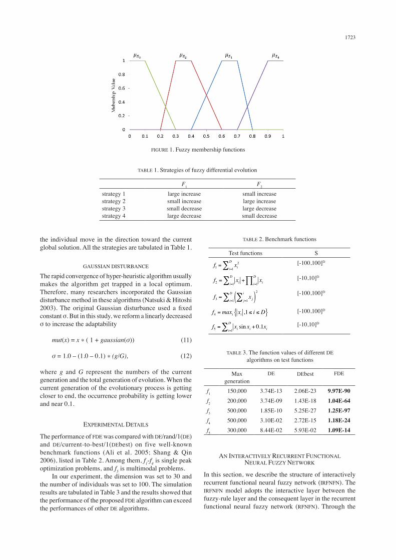
information sharing among the nodes in this layer, it can improve the overall performance of the network. Figure 2 illustrates the structure of the IRFNFN.

Layer 1: No function is performed in this layer. The node only transmits input values to layer 2.

ui(1) = xi. (13)

Layer 2: Nodes in this layer correspond to a single linguistic label of the input variables in layer 1.

ui(2) = oi

(1), (14)

hij(2) = exp (15)

where mij and σij are the mean and variance of the Gaussian membership function, respectively. Additionally, this layer also has a recurrent relationship.

oij(2)(t) = hij

(2)(t) + oij(2)(t – 1) .θij, (16)

where θij is the feedback weight.

Layer 3: Nodes in this layer are called rule nodes and the product operator is adopted to perform the precondition part of the fuzzy rules.

oj(3) = ∏iuij

(3). (17)

Layer 4: This layer is the interactive layer. Node can exchange information with other rule nodes,

(18)

(19)

where q and M represent for the number of output and the number of fuzzy rule; is the interactive influence weight; and Ok

(4) (t – 1) - k-th is the node’s previous output result.

Layer 5: Node in this layer received the output from layer 4 and the functional-link neural network (FLNN) output.

oj(5) = uj

(5) (20)

where wkj is the corresponding link weight of the FLNN and k is the functional expansion of input variables.

Layer 6: The output node acts as a defuzzifier with

(21)

where R is the number of fuzzy rules; and y is the output of IRFNFN model. The parameter optimization of IRFNFN is learned by the FDE learning algorithm, which has been mentioned previously.

FIGURE 2. Structure of IRFNFN model

1725

RESULTS

In order to determine the performance of the proposed approach, we compare the experimental results with other learning methods such as DE and DEbest. The scaling factor F and the population size play a pivotal role in guiding the convergence rate. There are two alternatives in choosing these two parameters: A population of large individuals with smaller F and a small population with F ≥ 0.8 (Montgomery 2010; Montgomery et al. 2010). In order to compromise between convergence speed and convergence probability, F = 0.9 is a good choice (Ronkkonen et al. 2005). In this study, we use a small population and set F=0.9. The default parameters are tabulated in Table 4.

system borders and surroundings. Assuming that TR and C are essentially constant, we rewrite the system in (23) into discrete-time form.

y(k + 1) = e–∝Tsy(k) + y(k) + [1 – e–αTs]y0,

(24)

where α and δ are constant values describing TR and C. The system parameters used in this example were α=1.0015e-4, δ=8.67973e-3, and Y0=25.0. The input u(k) was limited to 0 and 5V representing voltage units and the sampling period TS was set to 30. The 120 training patterns were chosen from the input-output characteristics in order to cover the entire reference output. In this experiment, we only use three fuzzy rules to control the water bath temperature system. The result of learning process is tabulated in Table 5. After the parameter optimization of IRFNFN is completed by the FDE learning, we test the network performance by the testing data

(25)

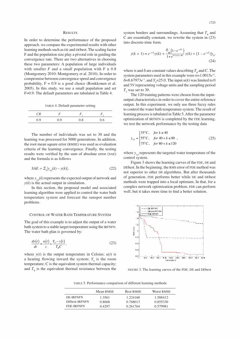
where yref represents the targeted water temperature of the control system. Figure 3 shows the learning curves of the FDE, DE and DEbest. In the beginning, the RMS error of FDE method was not superior to other DE algorithms. But after thousands of generation, FDE performs better while DE and DEbest methods were trapped into a local optimum. In that, for a complex network optimization problem, FDE can perform well, but it takes more time to find a better solution.

TABLE 4. Default parameter setting

CR F F1 F2

0.9 0.9 0.8 0.6

The number of individuals was set to 30 and the learning was processed for 5000 generations. In addition, the root mean square error (RMSE) was used as evaluation criteria of the learning convergence. Finally, the testing results were verified by the sum of absolute error (SAE) and the formula is as follows

SAE=Σk|yref(k) – y(k)|, (22)

where yref(k) represents the expected output of network and y(k) is the actual output in simulation. In this section, the proposed model and associated learning algorithm were applied to control the water bath temperature system and forecast the sunspot number problems.

CONTROL OF WATER BATH TEMPERATURE SYSTEM

The goal of this example is to adjust the output of a water bath system to a stable target temperature using the IRFNFN. The water bath plan is governed by:

(23)

where y(t) is the output temperature in Celsius; u(t) is a heating flowing inward the system; Y0 is the room temperature; C is the equivalent system thermal capacity; and TR is the equivalent thermal resistance between the

TABLE 5. Performance comparison of different learning methods

Mean RMSE Best RMSE Worst RMSE

DE-IRFNFNDEbest-IRFNFNFDE-IRFNFN

1.35610.86680.4297

1.2241600.7680130.261764

1.5884120.8553300.579981

FIGURE 3. The learning curves of the FDE, DE and DEbest

1726

The testing results of water bath temperature control system by using DE, DEbest and FDE learning methods are shown in Figure 4(a)-4(c). Figure 4(d) shows the temperature difference between the desired output and the model output. Table 6 shows the sum of absolute error (SAE) by using various learning methods. In this table, we can find that the SAE of FDE has the lowest value.

FORECAST OF THE SUNSPOT NUMBER

The sunspot numbers exhibit a nonlinear pattern and those are difficult to predict. The inputs x1 is defined as x1(t) = (t – 1), x2(t) = (t – 2) and x3(t) = (t – 3), where t represents the year and (t – 1) is the sunspot number at

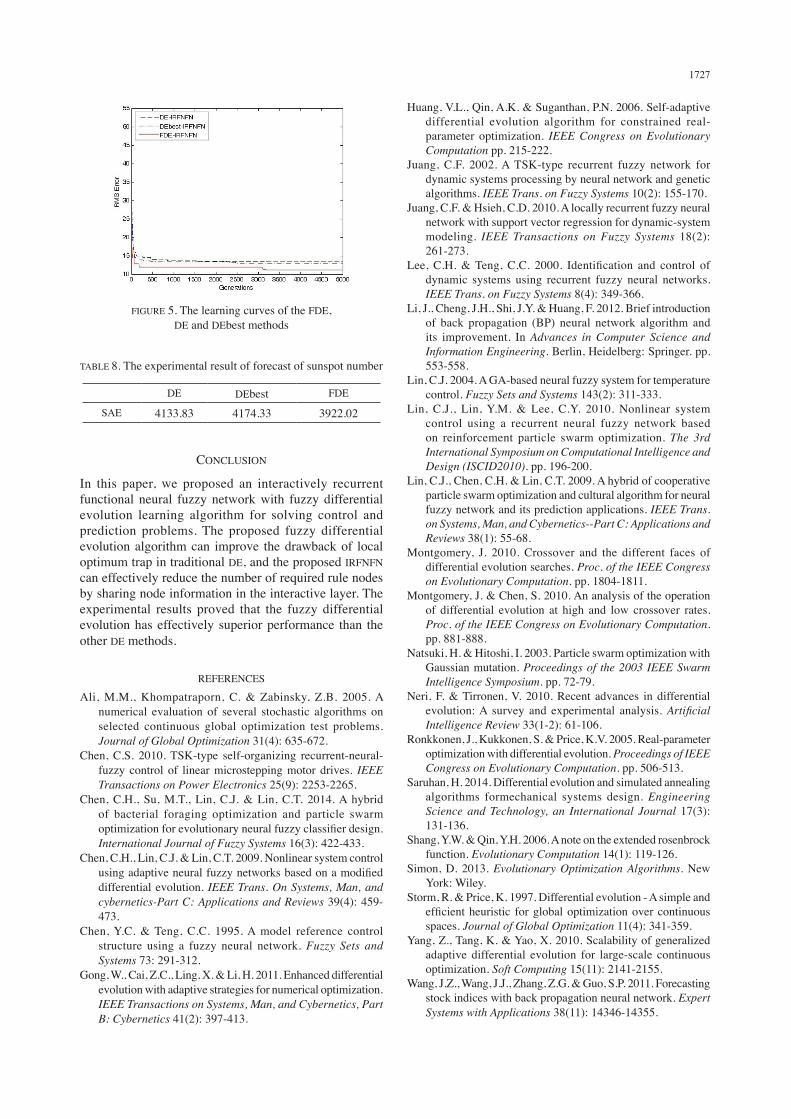
the t year. In this experiment, 151 data (from 1703 to 1884) were selected as the training set and the whole 302 data (from 1703 to 2004) were used as testing data. Here we use only three fuzzy rules to perform prediction problem. The experimental results using various learning methods are shown in Table 7. Figure 5 shows the learning curves of various learning methods. In this figure, we can see that DE and DEbest have fallen into the local optimum during the learning process. In contrast, the proposed FDE can escape from the local solution after 3000 iterations. Table 8 tabulates the sum of absolute error (SAE) by using various learning methods. The results showed that the proposed method has superior performances than the others.

TABLE 6. The experimental result of water bath temperature control system

DE DEbest FDE

SAE 474.252 422.966 404.207

TABLE 7. Performance comparison of various learning methods

Mean RMSE Best RMSE Worst RMSE

DE-IRFNFN 13.8941 13.3845 14.7746DEbest-IRFNFN 13.067 12.9121 13.4989FDE-IRFNFN 11.9511 11.1615 12.0102

FIGURE 4. The testing results of water bath temperature control system, (a) DE, (b) DEbest, (c) FDE and (d) temperature error

(a) (b)

(c) (d)

1727

CONCLUSION

In this paper, we proposed an interactively recurrent functional neural fuzzy network with fuzzy differential evolution learning algorithm for solving control and prediction problems. The proposed fuzzy differential evolution algorithm can improve the drawback of local optimum trap in traditional DE, and the proposed IRFNFN can effectively reduce the number of required rule nodes by sharing node information in the interactive layer. The experimental results proved that the fuzzy differential evolution has effectively superior performance than the other DE methods.

REFERENCES

Ali, M.M., Khompatraporn, C. & Zabinsky, Z.B. 2005. A numerical evaluation of several stochastic algorithms on selected continuous global optimization test problems. Journal of Global Optimization 31(4): 635-672.

Chen, C.S. 2010. TSK-type self-organizing recurrent-neural-fuzzy control of linear microstepping motor drives. IEEE Transactions on Power Electronics 25(9): 2253-2265.

Chen, C.H., Su, M.T., Lin, C.J. & Lin, C.T. 2014. A hybrid of bacterial foraging optimization and particle swarm optimization for evolutionary neural fuzzy classifier design. International Journal of Fuzzy Systems 16(3): 422-433.

Chen, C.H., Lin, C.J. & Lin, C.T. 2009. Nonlinear system control using adaptive neural fuzzy networks based on a modified differential evolution. IEEE Trans. On Systems, Man, and cybernetics-Part C: Applications and Reviews 39(4): 459-473.

Chen, Y.C. & Teng, C.C. 1995. A model reference control structure using a fuzzy neural network. Fuzzy Sets and Systems 73: 291-312.

Gong, W., Cai, Z.C., Ling, X. & Li, H. 2011. Enhanced differential evolution with adaptive strategies for numerical optimization. IEEE Transactions on Systems, Man, and Cybernetics, Part B: Cybernetics 41(2): 397-413.

Huang, V.L., Qin, A.K. & Suganthan, P.N. 2006. Self-adaptive differential evolution algorithm for constrained real-parameter optimization. IEEE Congress on Evolutionary Computation pp. 215-222.

Juang, C.F. 2002. A TSK-type recurrent fuzzy network for dynamic systems processing by neural network and genetic algorithms. IEEE Trans. on Fuzzy Systems 10(2): 155-170.

Juang, C.F. & Hsieh, C.D. 2010. A locally recurrent fuzzy neural network with support vector regression for dynamic-system modeling. IEEE Transactions on Fuzzy Systems 18(2): 261-273.

Lee, C.H. & Teng, C.C. 2000. Identification and control of dynamic systems using recurrent fuzzy neural networks. IEEE Trans. on Fuzzy Systems 8(4): 349-366.

Li, J., Cheng, J.H., Shi, J.Y. & Huang, F. 2012. Brief introduction of back propagation (BP) neural network algorithm and its improvement. In Advances in Computer Science and Information Engineering. Berlin, Heidelberg: Springer. pp. 553-558.

Lin, C.J. 2004. A GA-based neural fuzzy system for temperature control. Fuzzy Sets and Systems 143(2): 311-333.

Lin, C.J., Lin, Y.M. & Lee, C.Y. 2010. Nonlinear system control using a recurrent neural fuzzy network based on reinforcement particle swarm optimization. The 3rd International Symposium on Computational Intelligence and Design (ISCID2010). pp. 196-200.

Lin, C.J., Chen, C.H. & Lin, C.T. 2009. A hybrid of cooperative particle swarm optimization and cultural algorithm for neural fuzzy network and its prediction applications. IEEE Trans. on Systems, Man, and Cybernetics--Part C: Applications and Reviews 38(1): 55-68.

Montgomery, J. 2010. Crossover and the different faces of differential evolution searches. Proc. of the IEEE Congress on Evolutionary Computation. pp. 1804-1811.

Montgomery, J. & Chen, S. 2010. An analysis of the operation of differential evolution at high and low crossover rates. Proc. of the IEEE Congress on Evolutionary Computation. pp. 881-888.

Natsuki, H. & Hitoshi, I. 2003. Particle swarm optimization with Gaussian mutation. Proceedings of the 2003 IEEE Swarm Intelligence Symposium. pp. 72-79.

Neri, F. & Tirronen, V. 2010. Recent advances in differential evolution: A survey and experimental analysis. ArtificialIntelligence Review 33(1-2): 61-106.

Ronkkonen, J., Kukkonen, S. & Price, K.V. 2005. Real-parameter optimization with differential evolution. Proceedings of IEEE Congress on Evolutionary Computation. pp. 506-513.

Saruhan, H. 2014. Differential evolution and simulated annealing algorithms formechanical systems design. Engineering Science and Technology, an International Journal 17(3): 131-136.

Shang, Y.W. & Qin, Y.H. 2006. A note on the extended rosenbrock function. Evolutionary Computation 14(1): 119-126.

Simon, D. 2013. Evolutionary Optimization Algorithms. New York: Wiley.

Storm, R. & Price, K. 1997. Differential evolution - A simple and efficient heuristic for global optimization over continuous spaces. Journal of Global Optimization 11(4): 341-359.

Yang, Z., Tang, K. & Yao, X. 2010. Scalability of generalized adaptive differential evolution for large-scale continuous optimization. Soft Computing 15(11): 2141-2155.

Wang, J.Z., Wang, J.J., Zhang, Z.G. & Guo, S.P. 2011. Forecasting stock indices with back propagation neural network. Expert Systems with Applications 38(11): 14346-14355.

FIGURE 5. The learning curves of the FDE, DE and DEbest methods

TABLE 8. The experimental result of forecast of sunspot number

DE DEbest FDE

SAE 4133.83 4174.33 3922.02

1728

Cheng-Jian Lin*, Hsueh-Yi Lin & Cheng-Yi YuDepartment of Computer Science and Information EngineeringNational Chin-Yi University of TechnologyTaichung City 411 Taiwan, R.O.C.

Chih-Feng Wu

Department of Digital Content Application and ManagementWenzao Ursuline University of LanguagesKaohsiung City 807 Taiwan, R.O.C.

*Corresponding author; email: cjlin@ncut.edu.tw

Received: 22 August 2014Accepted: 23 June 2015