Support vector machines (SVMs) Lecture 6
David Sontag New York University
Slides adapted from Luke Zettlemoyer, Vibhav Gogate, and Carlos Guestrin
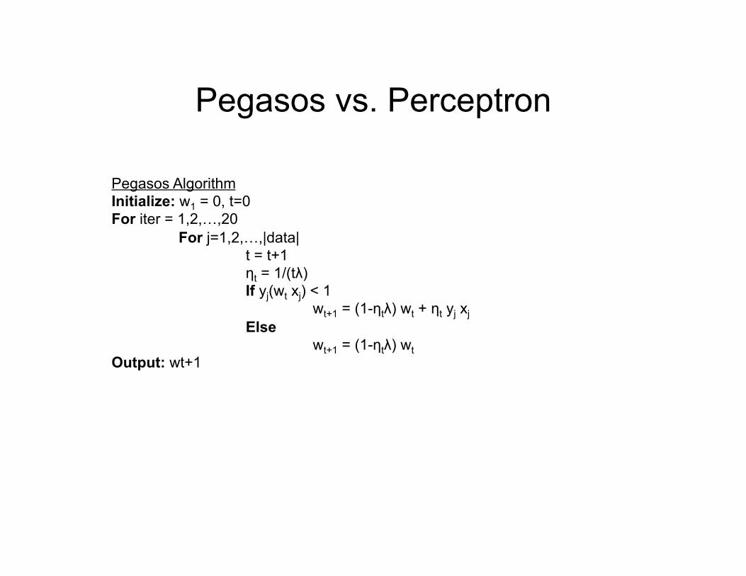
Pegasos vs. Perceptron
Pegasos Algorithm Initialize: w1 = 0, t=0 For iter = 1,2,…,20
For j=1,2,…,|data| t = t+1 ηt = 1/(tλ) If yj(wt xj) < 1 wt+1 = (1-ηtλ) wt + ηt yj xj Else wt+1 = (1-ηtλ) wt
Output: wt+1
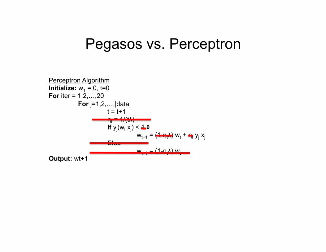
Pegasos vs. Perceptron
Perceptron Algorithm Initialize: w1 = 0, t=0 For iter = 1,2,…,20
For j=1,2,…,|data| t = t+1 ηt = 1/(tλ) If yj(wt xj) < 1 wt+1 = (1-ηtλ) wt + ηt yj xj Else wt+1 = (1-ηtλ) wt
Output: wt+1
0
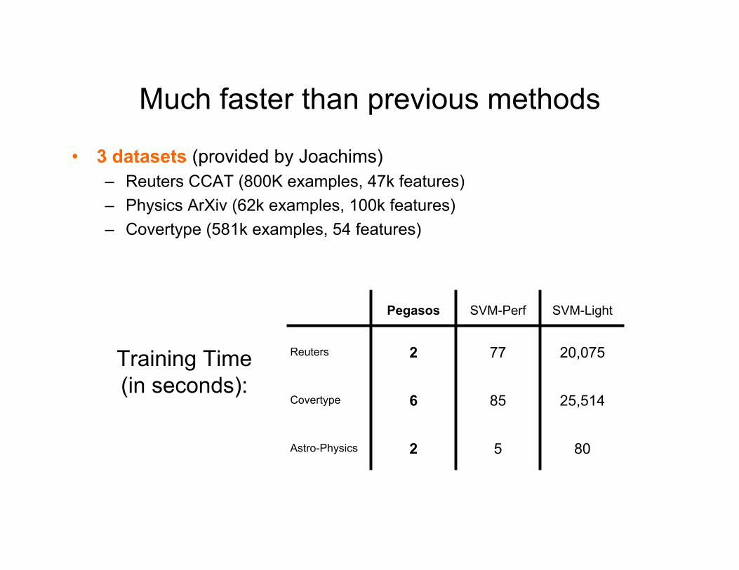
Much faster than previous methods
• 3 datasets (provided by Joachims) – Reuters CCAT (800K examples, 47k features) – Physics ArXiv (62k examples, 100k features) – Covertype (581k examples, 54 features)
Training Time (in seconds):
Pegasos SVM-Perf SVM-Light
Reuters 2 77 20,075
Covertype 6 85 25,514
Astro-Physics 2 5 80
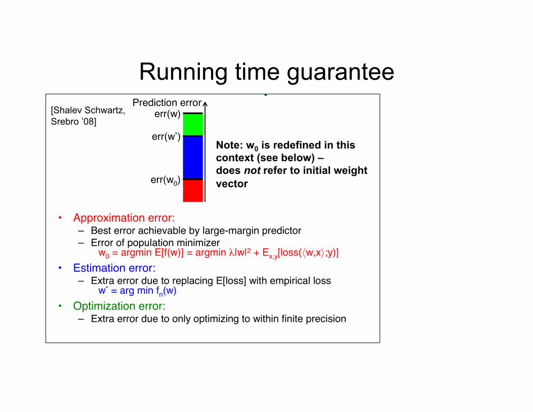
Running time guarantee Error Decomposition
• Approximation error:– Best error achievable by large-margin predictor– Error of population minimizer
w0 = argmin E[f(w)] = argmin λ|w|2 + Ex,y[loss(⟨w,x⟩;y)]• Estimation error:
– Extra error due to replacing E[loss] with empirical lossw* = arg min fn(w)
• Optimization error:– Extra error due to only optimizing to within finite precision
err(w0)
err(w*)
err(w)Prediction error
[Shalev Schwartz, Srebro ’08]
Note: w0 is redefined in this context (see below) – does not refer to initial weight vector
Error Decomposition
• Approximation error:– Best error achievable by large-margin predictor– Error of population minimizer
w0 = argmin E[f(w)] = argmin λ|w|2 + Ex,y[loss(⟨w,x⟩;y)]• Estimation error:
– Extra error due to replacing E[loss] with empirical lossw* = arg min fn(w)
• Optimization error:– Extra error due to only optimizing to within finite precision
err(w0)
err(w*)
err(w)Prediction error
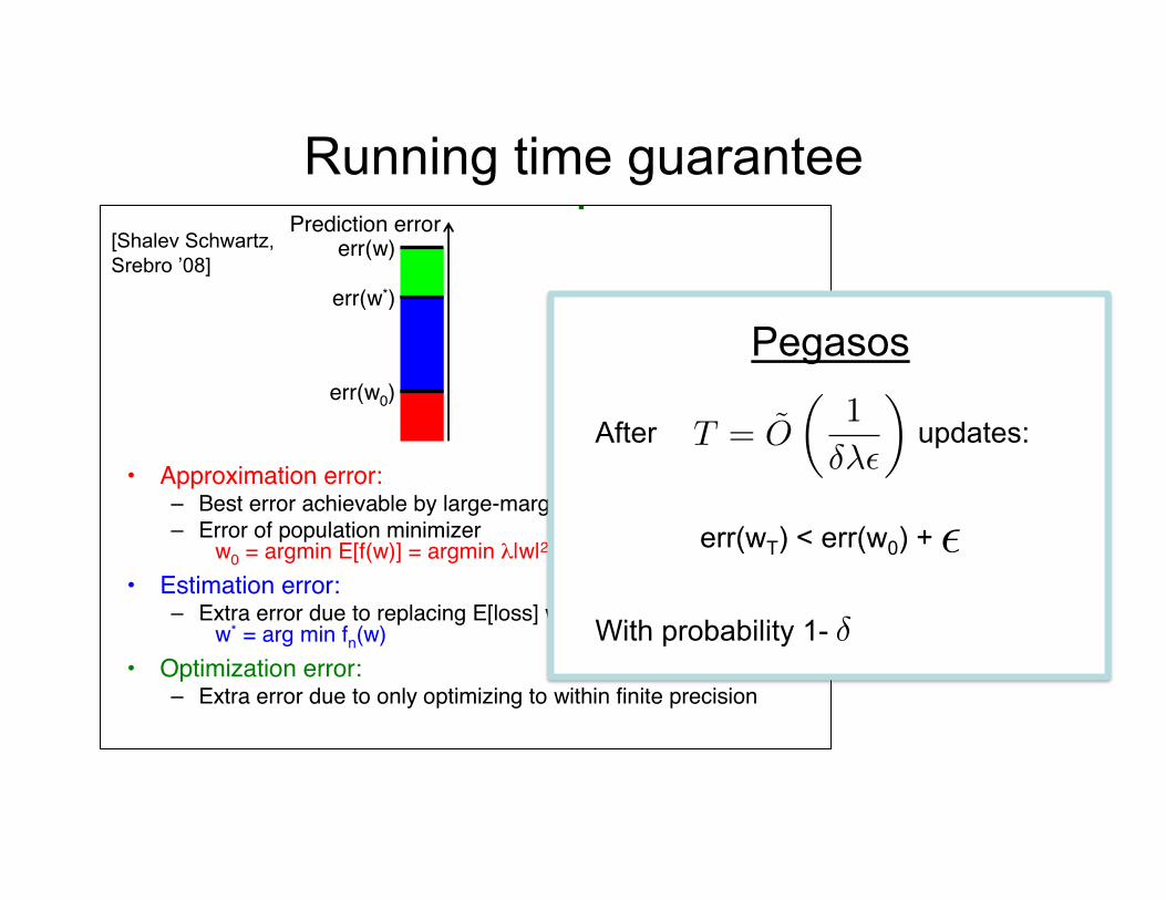
Pegasos
After updates:
err(wT) < err(w0) +
With probability 1-
✏
�
T = O
✓1
��✏
◆
Running time guarantee [Shalev Schwartz, Srebro ’08]
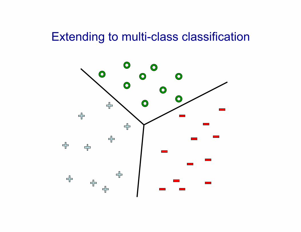
Extending to multi-class classification
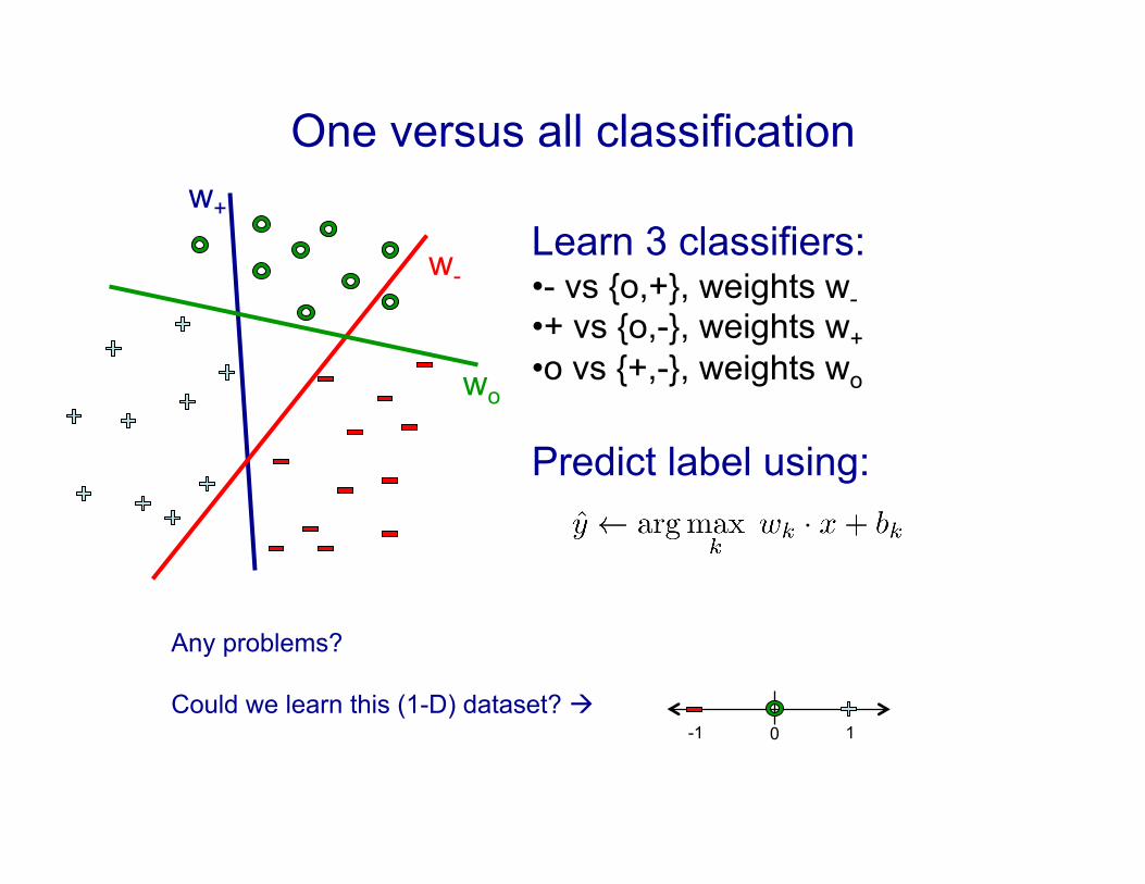
One versus all classification
Learn 3 classifiers: • - vs {o,+}, weights w- • + vs {o,-}, weights w+ • o vs {+,-}, weights wo
Predict label using:
w+
w-
Any problems?
Could we learn this (1-D) dataset? !
wo
0 -1 1
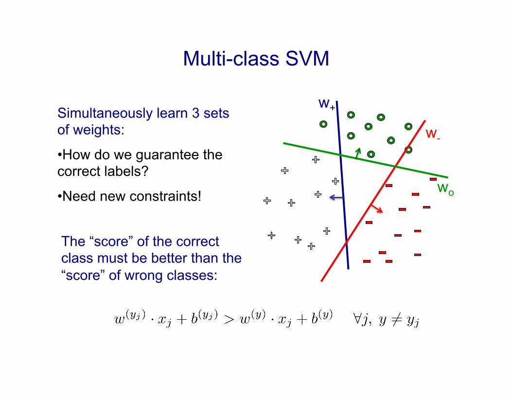
Multi-class SVM
Simultaneously learn 3 sets of weights:
• How do we guarantee the correct labels?
• Need new constraints!
w+
w-
wo
The “score” of the correct class must be better than the “score” of wrong classes:
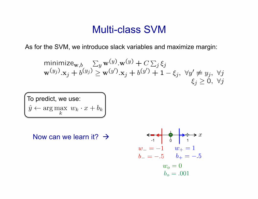
As for the SVM, we introduce slack variables and maximize margin:
Now can we learn it? !
Multi-class SVM
To predict, we use:
0 -1 1
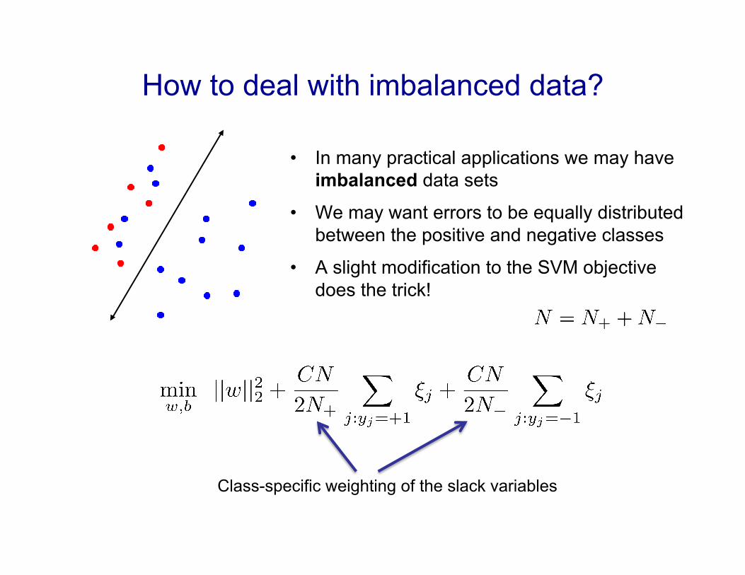
• In many practical applications we may have imbalanced data sets
• We may want errors to be equally distributed between the positive and negative classes
• A slight modification to the SVM objective does the trick!
How to deal with imbalanced data?
Class-specific weighting of the slack variables
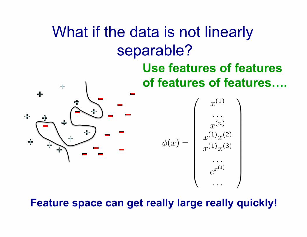
What if the data is not linearly separable?
Use features of features of features of features….
Feature space can get really large really quickly!
�(x) =
�
⇧⇧⇧⇧⇧⇧⇧⇧⇧⇧⇧⇤
x(1)
. . .x(n)
x(1)x(2)
x(1)x(3)
. . .
ex(1)
. . .
⇥
⌃⌃⌃⌃⌃⌃⌃⌃⌃⌃⌃⌅
7
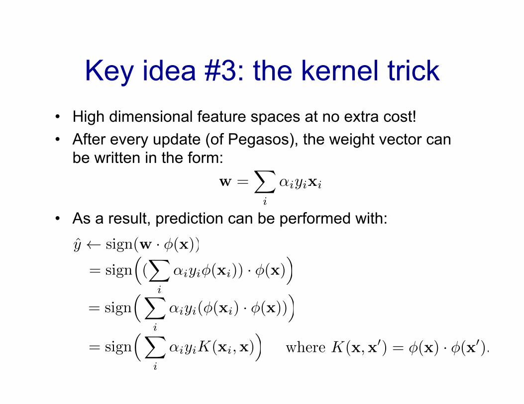
Key idea #3: the kernel trick • High dimensional feature spaces at no extra cost! • After every update (of Pegasos), the weight vector can
be written in the form:
• As a result, prediction can be performed with:
w =X
i
↵iyixi
= sign⇣X
i
↵iyiK(xi,x)⌘
= sign⇣X
i
↵iyi(�(xi) · �(x))⌘
= sign⇣(X
i
↵iyi�(xi)) · �(x)⌘y sign(w · �(x))
where K(x,x0) = �(x) · �(x0).
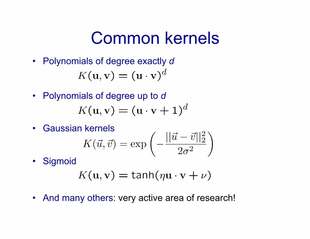
Common kernels • Polynomials of degree exactly d
• Polynomials of degree up to d
• Gaussian kernels
• Sigmoid
• And many others: very active area of research!
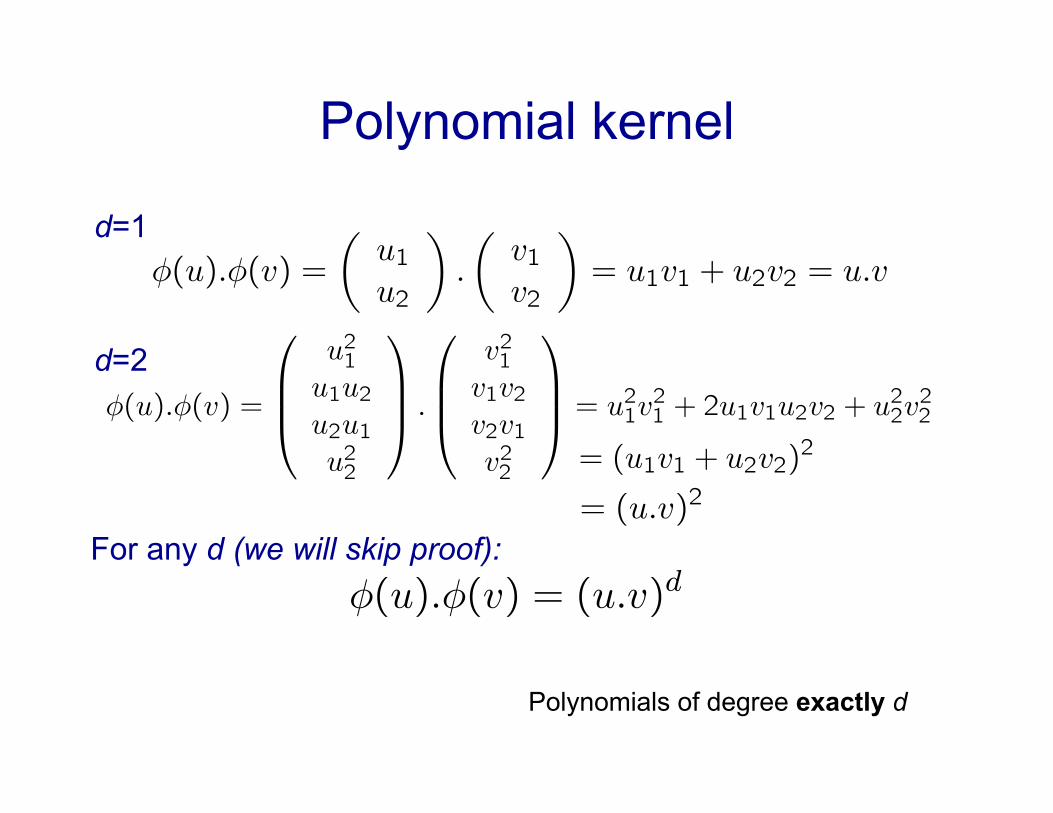
Polynomial kernel
Polynomials of degree exactly d
d=1
⇥(x) =
⇤
⌥⌥⌥⌥⌥⌥⌥⌥⌥⌥⌥⇧
x(1)
. . .x(n)
x(1)x(2)
x(1)x(3)
. . .
ex(1)
. . .
⌅
�����������⌃
⇤L
⇤w= w �
j
�jyjxj
⇥(u).⇥(v) =
�u1u2
⇥.
�v1v2
⇥= u1v1 + u2v2 = u.v
7
d=2
For any d (we will skip proof):
⇥(x) =
⇤
⌥⌥⌥⌥⌥⌥⌥⌥⌥⌥⌥⇧
x(1)
. . .x(n)
x(1)x(2)
x(1)x(3)
. . .
ex(1)
. . .
⌅
�����������⌃
⇤L
⇤w= w �
j
�jyjxj
⇥(u).⇥(v) =
�u1u2
⇥.
�v1v2
⇥= u1v1 + u2v2 = u.v
⇥(u).⇥(v) = (u.v)d
7
⇥(x) =
⇤
⌥⌥⌥⌥⌥⌥⌥⌥⌥⌥⌥⇧
x(1)
. . .x(n)
x(1)x(2)
x(1)x(3)
. . .
ex(1)
. . .
⌅
�����������⌃
⇤L
⇤w= w �
j
�jyjxj
⇥(u).⇥(v) =
�u1u2
⇥.
�v1v2
⇥= u1v1 + u2v2 = u.v
⇥(u).⇥(v) =
⇤
⌥⌥⇧
u21u1u2u2u1u22
⌅
��⌃ .
⇤
⌥⌥⇧
v21v1v2v2v1v22
⌅
��⌃ = u21v21 + 2u1v1u2v2 + u22v
22
⇥(u).⇥(v) = (u.v)d
7
⇥(x) =
⇤
⌥⌥⌥⌥⌥⌥⌥⌥⌥⌥⌥⇧
x(1)
. . .x(n)
x(1)x(2)
x(1)x(3)
. . .
ex(1)
. . .
⌅
�����������⌃
⇤L
⇤w= w �
j
�jyjxj
⇥(u).⇥(v) =
�u1u2
⇥.
�v1v2
⇥= u1v1 + u2v2 = u.v
⇥(u).⇥(v) =
⇤
⌥⌥⇧
u21u1u2u2u1u22
⌅
��⌃ .
⇤
⌥⌥⇧
v21v1v2v2v1v22
⌅
��⌃ = u21v21 + 2u1v1u2v2 + u22v
22
= (u1v1 + u2v2)2
⇥(u).⇥(v) = (u.v)d
7
⇥(x) =
⇤
⌥⌥⌥⌥⌥⌥⌥⌥⌥⌥⌥⇧
x(1)
. . .x(n)
x(1)x(2)
x(1)x(3)
. . .
ex(1)
. . .
⌅
�����������⌃
⇤L
⇤w= w �
j
�jyjxj
⇥(u).⇥(v) =
�u1u2
⇥.
�v1v2
⇥= u1v1 + u2v2 = u.v
⇥(u).⇥(v) =
⇤
⌥⌥⇧
u21u1u2u2u1u22
⌅
��⌃ .
⇤
⌥⌥⇧
v21v1v2v2v1v22
⌅
��⌃ = u21v21 + 2u1v1u2v2 + u22v
22
= (u1v1 + u2v2)2
= (u.v)2
⇥(u).⇥(v) = (u.v)d
7
[Tommi Jaakkola]
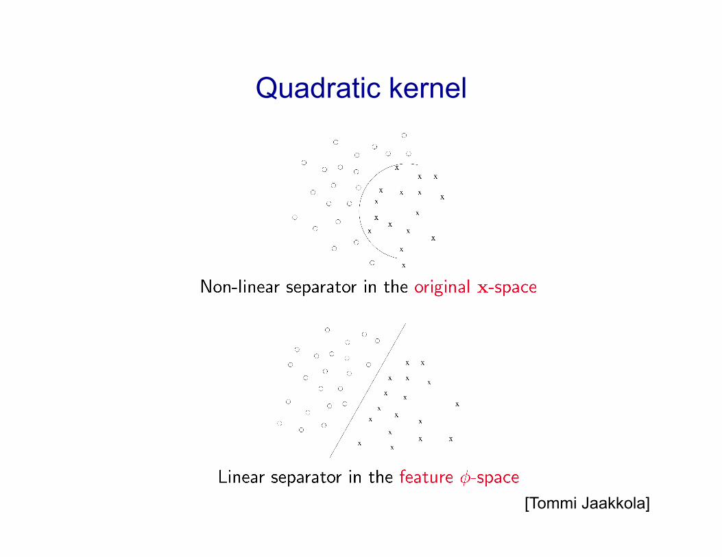
Quadratic kernel
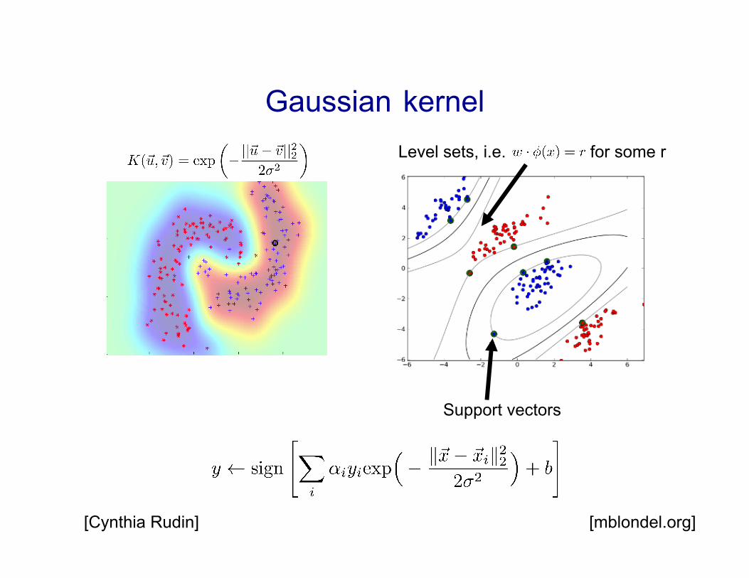
Gaussian kernel
[Cynthia Rudin] [mblondel.org]
Support vectors
Level sets, i.e. for some r
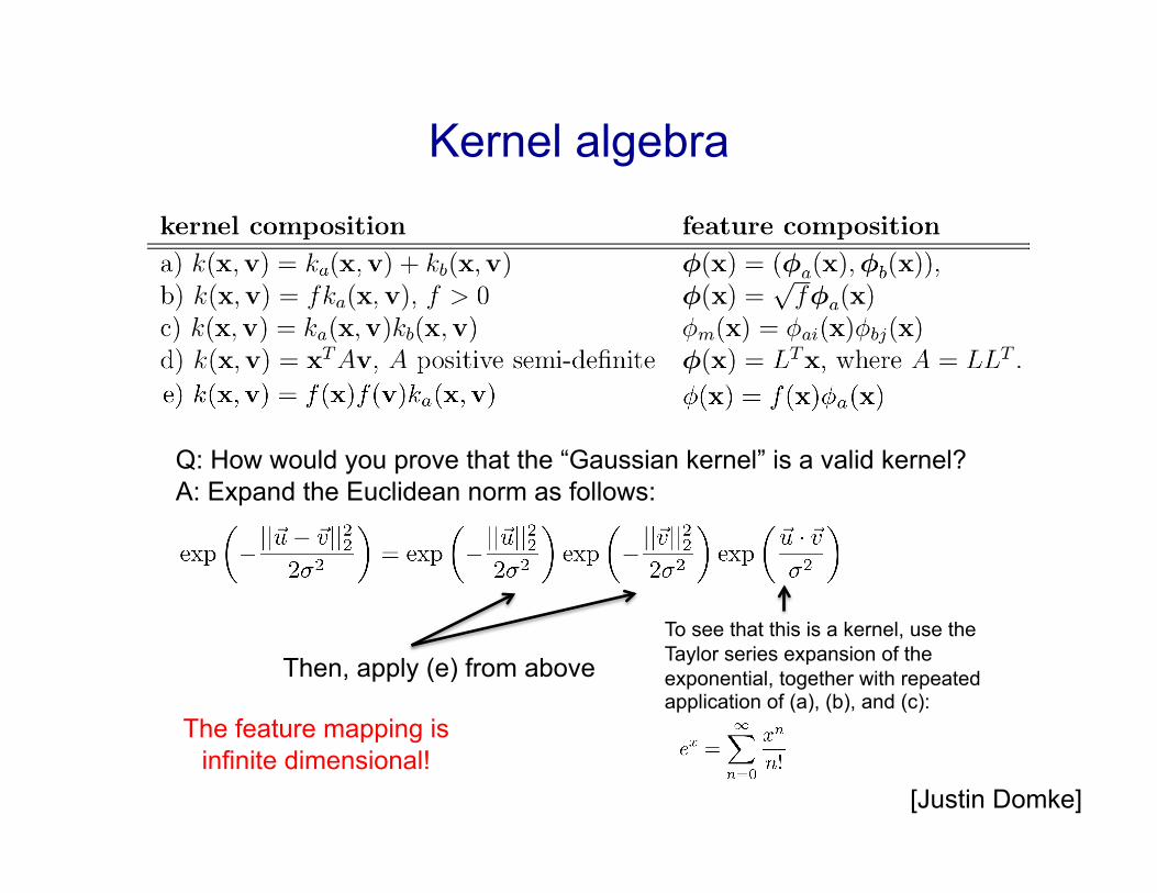
Kernel algebra
[Justin Domke]
Q: How would you prove that the “Gaussian kernel” is a valid kernel? A: Expand the Euclidean norm as follows:
Then, apply (e) from above To see that this is a kernel, use the Taylor series expansion of the exponential, together with repeated application of (a), (b), and (c):
The feature mapping is infinite dimensional!
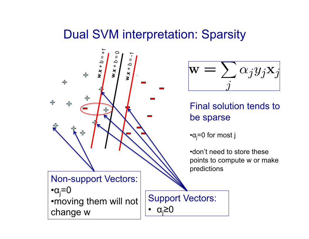
Dual SVM interpretation: Sparsity
w.x
+ b
= +
1
w.x
+ b
= -1
w.x
+ b
= 0
Support Vectors: • αj≥0
Non-support Vectors: • αj=0 • moving them will not change w
Final solution tends to be sparse
• αj=0 for most j
• don’t need to store these points to compute w or make predictions
Overfitting?
• Huge feature space with kernels: should we worry about overfitting? – SVM objective seeks a solution with large margin
• Theory says that large margin leads to good generalization (we will see this in a couple of lectures)
– But everything overfits sometimes!!!
– Can control by: • Setting C
• Choosing a better Kernel
• Varying parameters of the Kernel (width of Gaussian, etc.)


