Download - Feature Lucas-Kanade(LK) Image Registration & Tracking ...faculty.petra.ac.id/resmana/private/compvision/slides/lucaskanade...• Extraksi feature dengan metode LK ini adalah sangat

1

Image Registration & Tracking dengan Metode Lucas & Kanade

Sumber:-Forsyth & Ponce Chap. 19, 20-Tomashi & Kanade: Good Feature to Track

Feature Lucas-Kanade(LK)

• Extraksi feature dengan metode LK ini adalahsangat populer dalam aplikasi computer vision.

• Feature diekstraksi dengan mengambil informasigradient image.

• Selanjutnya feature ini bisa dimanfaatkan untukImage registration, yg. Selanjutnya diugnakan utk. tracking, recognition, dan lain-lain

• Pemilihan feature image yang tepat adalah sangatmenentukan keberhasilan proses recognition, tracking, etc.

Sejarah Perkembangan LK

• Lucas & Kanade (IUW 1981)

LK BAHH ST S BJ HB BL G SI CETSC

• Bergen, Anandan, Hanna, Hingorani (ECCV 1992)

• Shi & Tomasi (CVPR 1994)

• Szeliski & Coughlan (CVPR 1994)

• Szeliski (WACV 1994)

• Black & Jepson (ECCV 1996)

• Hager & Belhumeur (CVPR 1996)

• Bainbridge-Smith & Lane (IVC 1997)

• Gleicher (CVPR 1997)

• Sclaroff & Isidoro (ICCV 1998)

• Cootes, Edwards, & Taylor (ECCV 1998)

Image Registration

2

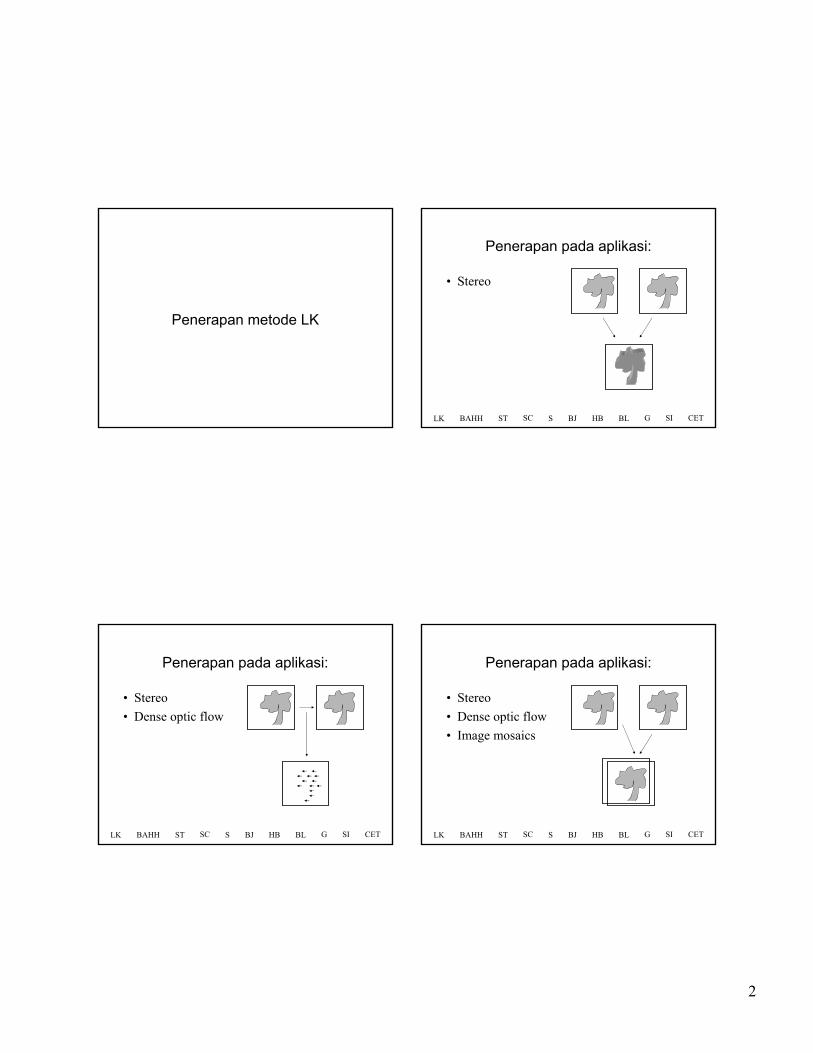
Penerapan metode LK

Penerapan pada aplikasi:

• Stereo



• Stereo

• Dense optic flow



• Stereo


• Image mosaics


3


• Stereo


• Image mosaics

• Tracking



• Stereo


• Image mosaics

• Tracking

• Recognition


?

Derivasi RumusanLucas & Kanade

#1

rumusan L&K 1

I0(x)

)('0 xI

h

xIhxIh

)()(lim 00

0

−+=

→

)('0 xI

4

rumusan L&K 1

)('0 xI

h

xIhxI )()( 00 −+≈

h I0(x)

I0(x+h)

rumusan L&K 1

h I0(x)

)('0 xI

h

xIxI )()( 0−≈

I(x)

rumusan L&K 1

h I0(x)

h)(

)()('0

0

xI

xIxI −≈

I(x)

rumusan L&K 1

I0(x)

h ∑∈

−≈

Rx xI

xIxI

R )(

)()(

||

1'0

0

RI(x)

5

rumusan L&K 1

I0(x)

h ∑∑ ∈

−≈

RxxxI

xIxIxw

xw )(

)]()()[(

)(

1'0

0

I(x)

rumusan L&K 1

h0 I0(x)

0h

I(x)

∑∑ ∈

−←

RxxxI

xIxIxw

xw )(

)]()()[(

)(

1'0

0

rumusan L&K 1

1h ∑∑ ∈ ++−

+←Rxx

hxI

hxIxIxw

xwh

)(

)]()()[(

)(

1

0'0

000

I0(x+h0)

I(x)

rumusan L&K 1

2h ∑∑ ∈ ++−

+←Rxx

hxI

hxIxIxw

xwh

)(

)]()()[(

)(

1

1'0

101

I0(x+h1)

I(x)

6

rumusan L&K 1

1+kh ∑∑ ∈ ++−

+←Rx k

k

x

k hxI

hxIxIxw

xwh

)(

)]()()[(

)(

1'0

0

I0(x+hk)

I(x)

rumusan L&K 1

1+kh ∑∑ ∈ ++−

+←Rx k

k

x

k hxI

hxIxIxw

xwh

)(

)]()()[(

)(

1'0

0

I0(x+hf)

I(x)

Derivasi RumusanLucas & Kanade

#2

rumusan L&K 2

• Sum-of-squared-difference (SSD) error

E(h) = Σ [ I(x) - I0(x+h) ]2x ε R

E(h) Σ [ I(x) - I0(x) - hI0’(x) ]2x ε R

≈

7

rumusan L&K 2

Σ 2[I0’(x)(I(x) - I0(x) ) - hI0’(x)2] x ε Rh

E

∂∂ ≈

Σ I0’(x)(I(x) - I0(x))x ε Rh ≈

Σ I0’(x)2x ε R

= 0

Perbandingan

Σ I0’(x)[I(x) - I0(x)]h ≈ Σ I0’(x)2

x

x

≈h

w(x)[I(x) - I0(x)]

Σ w(x)x

xΣ I0’(x)

Perbandingan

Σ I0’(x)[I(x) - I0(x)]h ≈ Σ I0’(x)2

x

≈h

x

w(x)[I(x) - I0(x)]

Σ w(x)x

xΣ I0’(x)Generalisasi metode Lucas-

Kanade

8

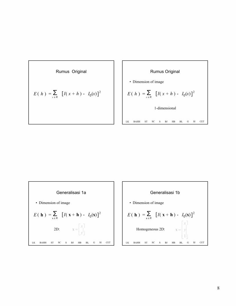
Rumus Original

h ) = Σx ε R

(E [I( x ) - (x ]2)+ h I0

Rumus Original

• Dimension of image

h ) = Σx ε R

(E [I( x ) - (x ]2)+ h

1-dimensional

I0


Generalisasi 1a


h ) = Σx ε R

(E [I( x ) - (x ]2)+ h

=

y

xx2D:

I0


Generalisasi 1b


h ) = Σx ε R

(E [I( x ) - (x ]2)+ h

=

1

y

x

xHomogeneous 2D:

I0


9

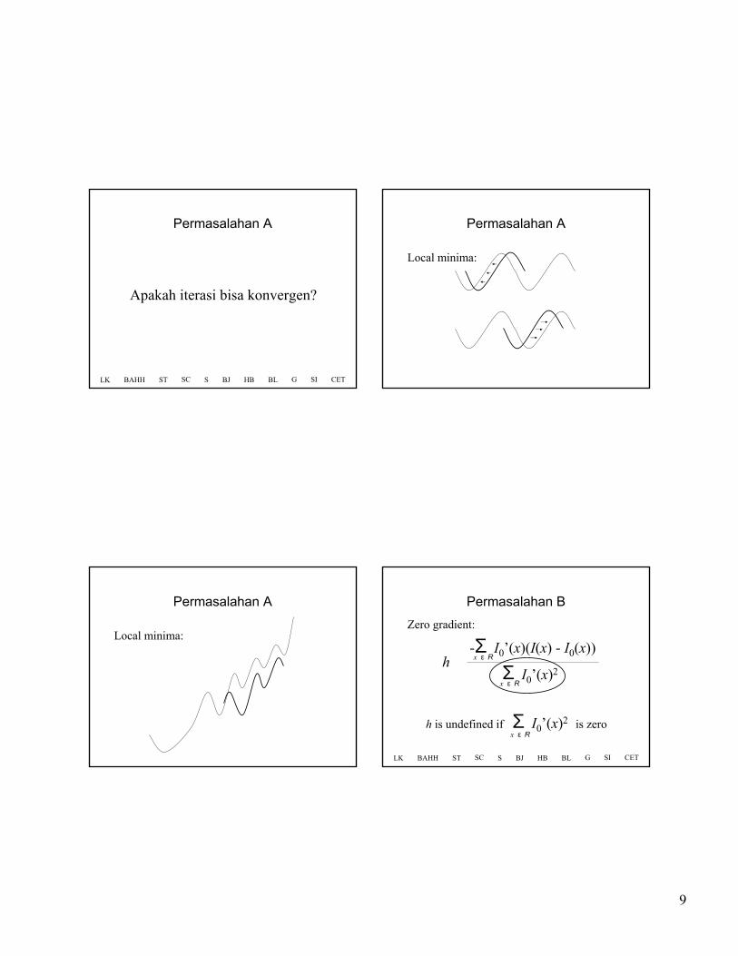
Permasalahan A


Apakah iterasi bisa konvergen?

Permasalahan A

Local minima:

Permasalahan A

Local minima:

Permasalahan B

-Σ I0’(x)(I(x) - I0(x))x ε Rh ≈

Σ I0’(x)2x ε R

h is undefined if Σ I0’(x)2 is zerox ε R


Zero gradient:

10

Permasalahan B

Zero gradient:

?

Permasalahan B’

-Σ (x)(I(x) - I0(x))x ε R

hy≈ Σ 2

x ε R

∂

∂y

I )(0 xy

I

∂∂ )(0 x

Aperture problem (mis. Image datar):


Permasalahan B’

No gradient along one direction:

?

Jawaban problem A & B

• Possible solutions:– Manual intervention


11


– Zero motion default





– Coefficient “dampening”






– Reliance on good features







– Temporal filtering



12






– Spatial interpolation / hierarchical estimation








– Spatial interpolation / hierarchical estimation

– Higher-order terms



Kembali lagi: Rumus Original

h ) = Σx ε R

(E [I( x ) - (x ]2)+ h I0

Rumus Original

• Transformations/warping of image

h ) = Σx ε R

(E [I( x ) - I0(x ]2)+ h

Translations:

=

y

x

δδ

h


13

Permasalahan C

Bagaimana bila ada gerakan(motion) tipe lain?

Generalisasi 2a


A, h) = Σx ε R

(E [I(Ax ) - (x ]2)+h

Affine:

=

dc

baA

=

y

x

δδ

h

I0


Generalisasi 2a

Affine:

=

dc

baA

=

y

x

δδ

h

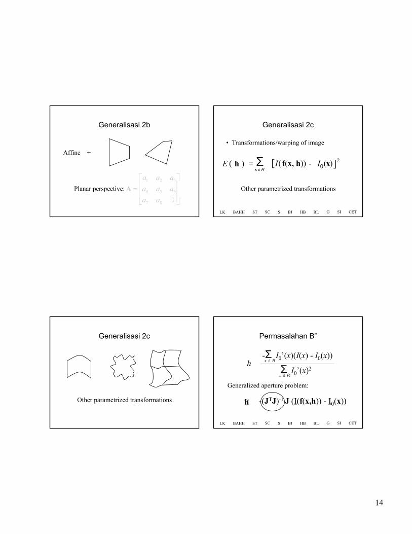
Generalisasi 2b


A ) = Σx ε R

(E [I( A x ) - (x ]2)

Planar perspective:

=

187

654

321

aa

aaa

aaa

A

I0


14

Generalisasi 2b

Planar perspective:

=

187

654

321

aa

aaa

aaa

A

Affine +

Generalisasi 2c


h ) = Σx ε R

(E [I( f(x, h)) - (x ]2)

Other parametrized transformations

I0


Generalisasi 2c

Other parametrized transformations

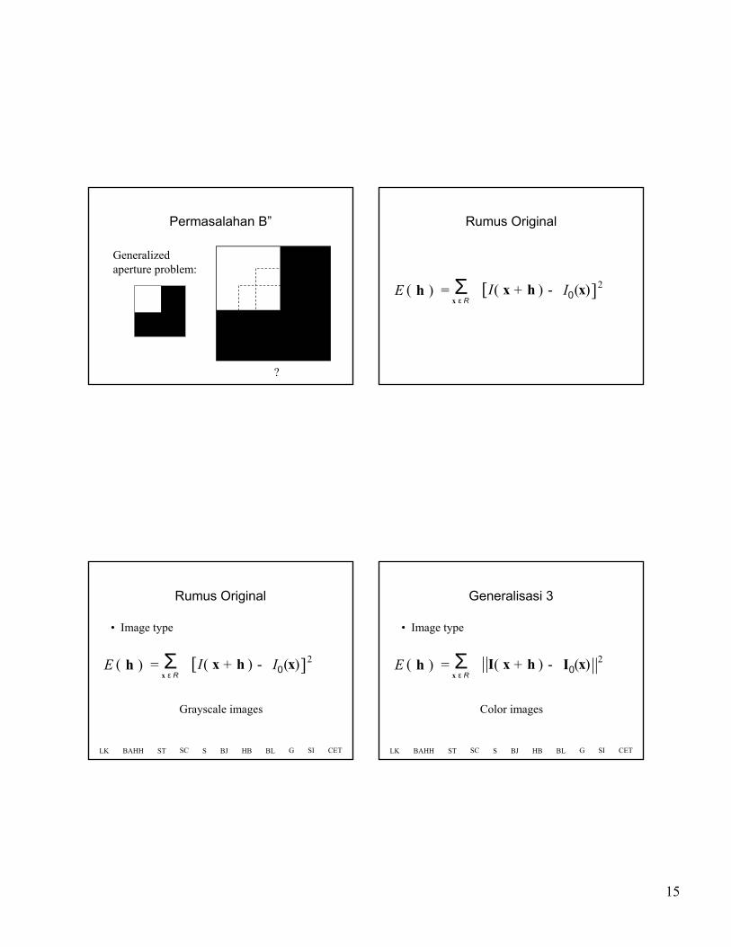
Permasalahan B”

-(JTJ)-1 J (I(f(x,h)) - I0(x))h ≈~

Generalized aperture problem:


-Σ I0’(x)(I(x) - I0(x))x ε Rh ≈

Σ I0’(x)2x ε R

15

Permasalahan B”

?

Generalizedaperture problem:

Rumus Original

h ) = Σx ε R

(E [I( x ) - (x ]2)+ h I0

Rumus Original

• Image type

h ) = Σx ε R

(E [I( x ) - (x ]2)+ h

Grayscale images

I0


Generalisasi 3

• Image type

h ) = Σx ε R

(E ||I( x ) - I0(x ||2)+ h

Color images


16

Rumus Original

h ) = Σx ε R

(E [I( x ) - (x ]2)+ h I0

Rumus Original

• Anggapan pixel punya konstan brightness (Constancy assumption)

h ) = Σx ε R

(E [I( x ) - I0(x ]2)+ h

Brightness constancy


Permasalahan C

Bagaimana bila iluminasi cahaya bervariasi?

Generalisasi 4a

• Constancy assumption

h,α,β )=Σx ε R

(E [I( x ) - αI0(x ]2)+β+ h

Linear brightness constancy


17

Generalisasi 4a Generalisasi 4b


h,λ) = Σx ε R

(E [I( x ) - λΤB(x]2)+ h

Illumination subspace constancy


Permasalahan C’

Bagaimana bila texture berubah?

Generalisasi 4c


h,λ) = Σx ε R

(E [I( x ) - ]2+ h

Texture subspace constancy

λΤB(x)


18

Permasalahan D

Jelas proses konvergensi menjadilambat bila jumlah #parameters

bertambah !!!

• Percepat konvergensi dengan:– Coarse-to-fine, filtering, interpolation, etc.


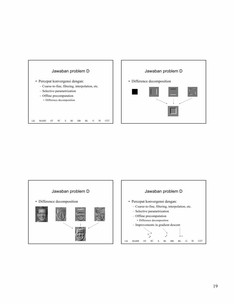
Jawaban problem D


– Selective parametrization

Jawaban problem D




– Offline precomputation

Jawaban problem D


19



– Offline precomputation• Difference decomposition

LK BAHH ST S BJ HB G SI CETSC

Jawaban problem D

BL

Jawaban problem D

• Difference decomposition

Jawaban problem D

• Difference decomposition • Percepat konvergensi dengan:– Coarse-to-fine, filtering, interpolation, etc.



– Improvements in gradient descent


Jawaban problem D

BL

20




– Improvements in gradient descent• Multiple estimates of spatial derivatives


Jawaban problem D

BL

Jawaban problem D

• Multiple estimates / state-space sampling

Generalisasi metode Lucas-Kanade

Σx ε R

[I( x ) - (x ]2)+ h I0

Modifikasi yg. Dibuat selama ini adalah:

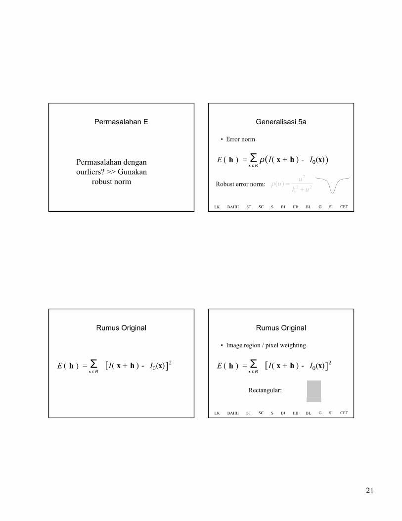
Rumus Original

• Error norm

h ) = Σx ε R

(E [I( x ) - I0(x ]2)+ h

Squared difference:


21

Permasalahan E

Permasalahan denganourliers? >> Gunakan

robust norm

Generalisasi 5a

• Error norm

h ) = Σx ε R

(E (I( x ) - I0(x ))+ h

Robust error norm:

ρ

22

2

)(uk

uuρ

+=


Rumus Original

h ) = Σx ε R

(E [I( x ) - (x ]2)+ h I0

Rumus Original

• Image region / pixel weighting

h ) = Σx ε R

(E [I( x ) - I0(x ]2)+ h

Rectangular:


22

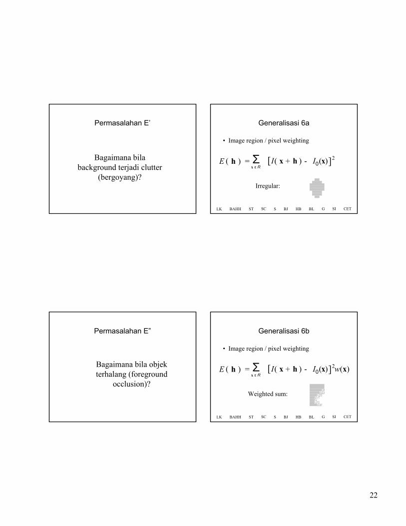
Permasalahan E’

Bagaimana bilabackground terjadi clutter

(bergoyang)?

Generalisasi 6a


h ) = Σx ε R

(E [I( x ) - I0(x ]2)+ h

Irregular:


Permasalahan E”

Bagaimana bila objekterhalang (foreground

occlusion)?

Generalisasi 6b


h ) = Σx ε R

(E [I( x ) - I0(x ]2)+ h

Weighted sum:

w(x)


23

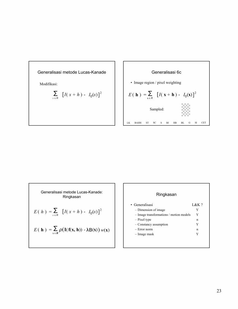
Generalisasi metode Lucas-Kanade

Σx ε R

[I( x ) - (x ]2)+ h I0

Modifikasi:

Generalisasi 6c


h ) = Σx ε R

(E [I( x ) - I0(x ]2)+ h

Sampled:


Generalisasi metode Lucas-Kanade: Ringkasan

= Σx ε R

(I( ) - w(x)ρ λΒ(x ))h )(E f(x, h)

h ) = Σx ε R

(E [I( x ) - (x ]2)+ h I0

Ringkasan

• Generalisasi– Dimension of image

– Image transformations / motion models

– Pixel type

– Constancy assumption

– Error norm

– Image mask

L&K ?Y

Y

n

Y

n

Y

24

Ringkasan

• Common problems:– Local minima

– Aperture effect

– Illumination changes

– Convergence issues

– Outliers and occlusions

L&K ?Y

maybe

Y

Y

n

Penanganan aperture effect:– Manual intervention



– Elimination of poor textures


– Spatial interpolation / hierarchical

– Higher-order terms

Ringkasan

L&K ?n

n

n

n

Y

Y

n

Download - Feature Lucas-Kanade(LK) Image Registration & Tracking ...faculty.petra.ac.id/resmana/private/compvision/slides/lucaskanade...• Extraksi feature dengan metode LK ini adalah sangat

Top Related