analisis deret waktu - pikasilvianti.staff.ipb.ac.id · ¾harga saham p.t. telkom di bej dari 2...

25/02/2015

1

Analisis Deret Waktu

Pertemuan 2

FMA, PKS. Dept. Statistika IPB

Jenis Data

• Cross sectionBeberapa pengamatan diamati bersama‐sama pada periode waktu tertentup p g p pHarga saham semua perusahaan yang tercatat di BEJ pada hari Rabu 27 Februari 2008

• Time SeriesSatu pengamatan diamati selama sekian periode secara teraturHarga saham P.T. TELKOM di BEJ dari 2 Januari 2008 hingga 27 Februari 2008

• Longitudinal/panelBeberapa pengamatan diamati bersama‐sama selama kurun waktu tertentu p p g(gabungan cross section dan time series)Harga saham P.T. TELKOM, P.T. INDOSAT, dan P.T. Mobile8 di BEJ dari 2 Januari 2008 hingga 27 Februari 2008


25/02/2015

2

Pola Data Time Series

5

6

7

8

9

30

35

40

45

50

0

1

2

3

4

5

1 2 3 4 5 6 7 8 9 10 11 12 13 14 15 16 17 18 19 20 21 22 23 24 25 26 27 28 29 30 31 32 33 34 35 36 0

5

10

15

20

25

1 2 3 4 5 6 7 8 9 10 11 12 13 14 15 16 17 18 19 20 21 22 23 24 25 26 27 28 29 30 31 32 33 34 35 36

14

16

18

20

25

Konstan Trend


0

2

4

6

8

10

12

1 2 3 4 5 6 7 8 9 10 11 12 13 14 15 16 17 18 19 20 21 22 23 24 25 26 27 28 29 30 31 32 33 34 35 360

5

10

15

1 2 3 4 5 6 7 8 9 10 11 12 13 14 15 16 17 18 19 20 21 22 23 24 25 26 27 28 29 30 31 32 33 34 35 36

Seasonal Cyclic

Metode Forecasting

Metode forecasting dapat dibedakan menjadi dua kelompok:dua kelompok:•Smoothing

Moving average, Single Exponential Smoothing, Double Exponential Smoothing, Metode Winter

•Modeling/ARIMA, ARCH/GARCH


25/02/2015

3

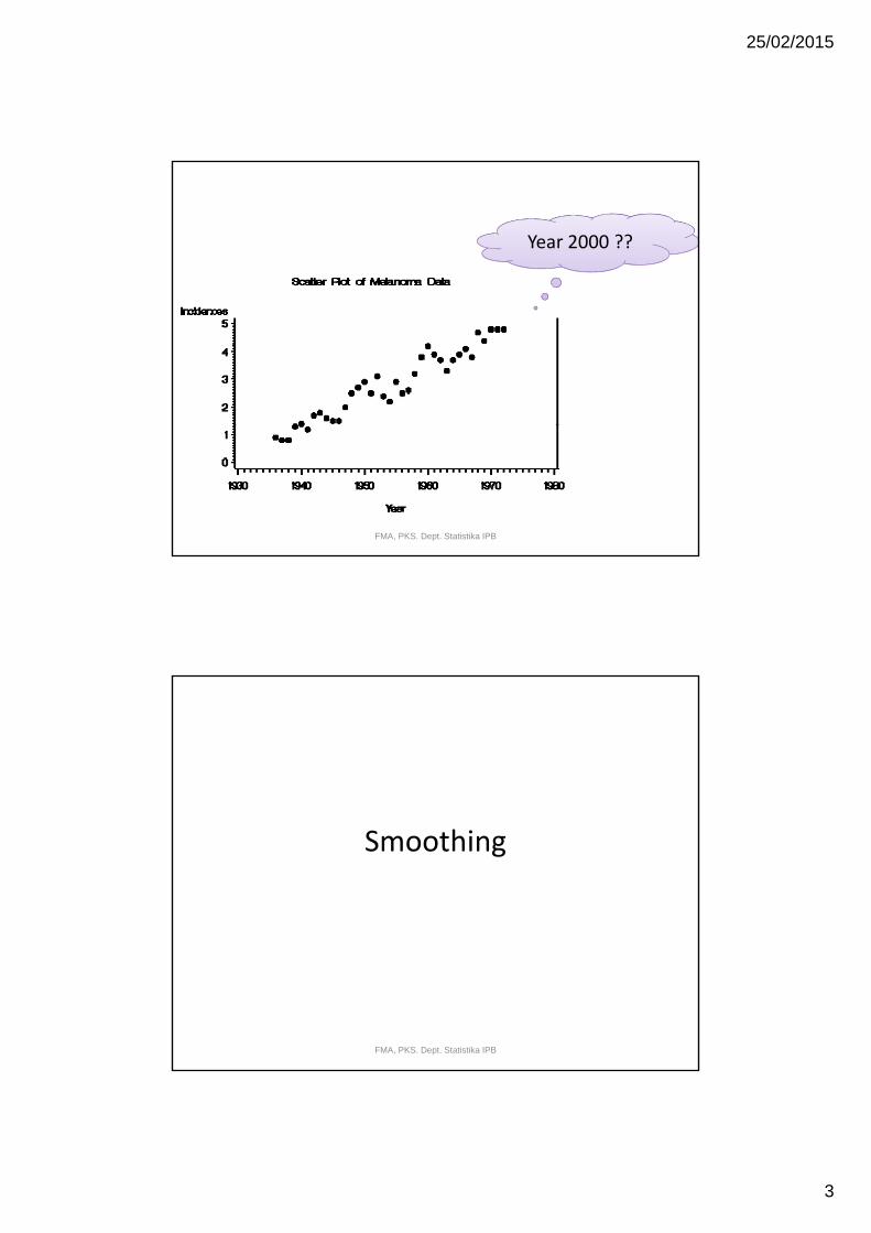
Year 2000 ??


Smoothing


25/02/2015

4

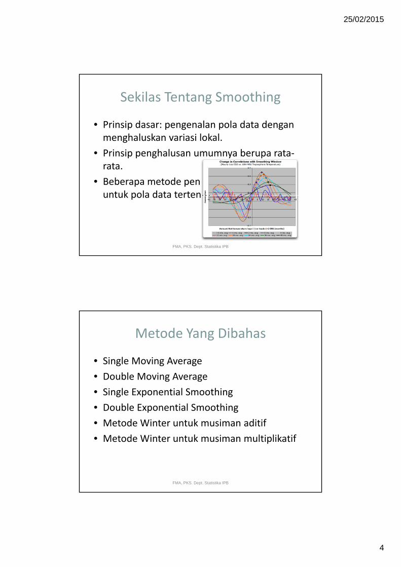
Sekilas Tentang Smoothing

• Prinsip dasar: pengenalan pola data dengan h l k i i l k lmenghaluskan variasi lokal.

• Prinsip penghalusan umumnya berupa rata‐rata.

• Beberapa metode penghalusan hanya cocok untuk pola data tertentuuntuk pola data tertentu.


Metode Yang Dibahas

• Single Moving Average• Double Moving Average• Single Exponential Smoothing• Double Exponential Smoothing• Metode Winter untuk musiman aditif• Metode Winter untuk musiman multiplikatif


25/02/2015

5

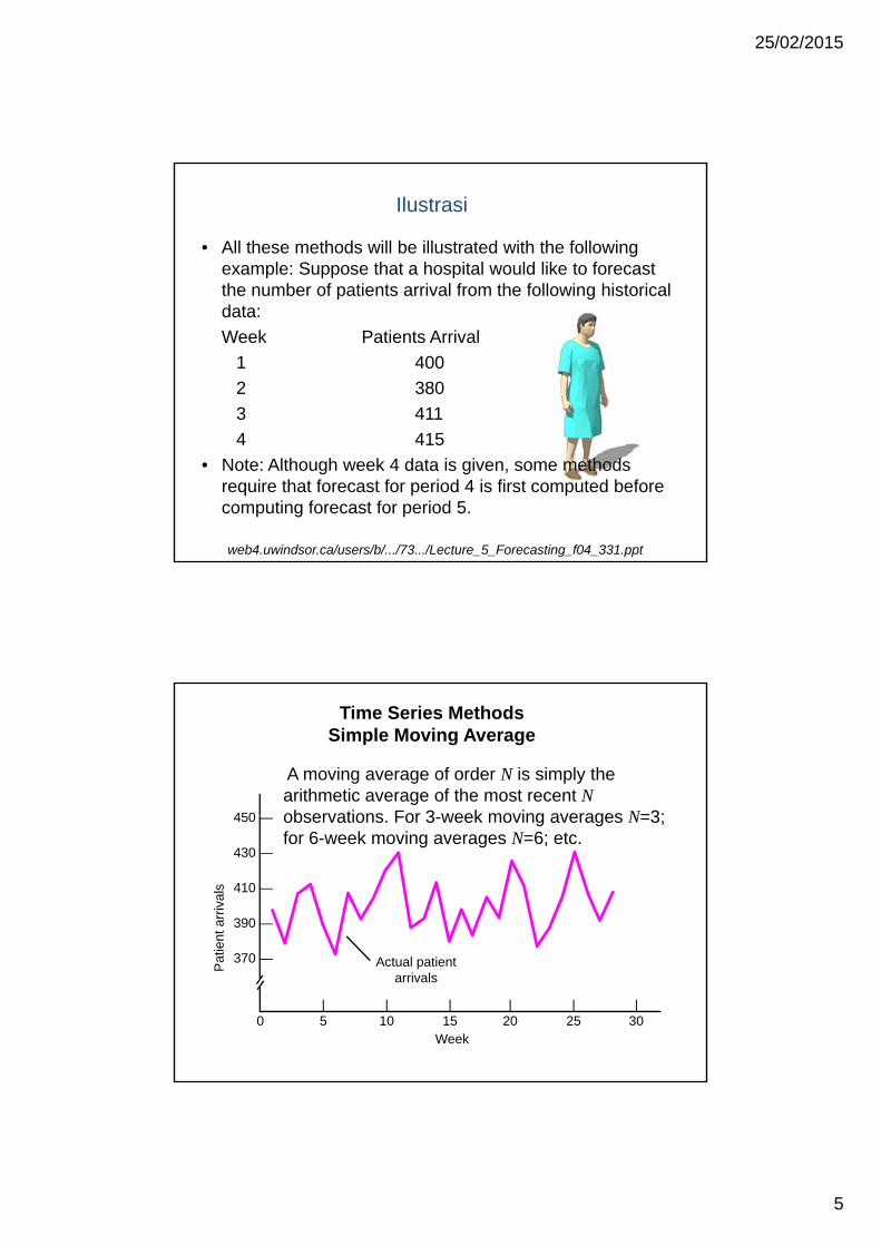
Ilustrasi

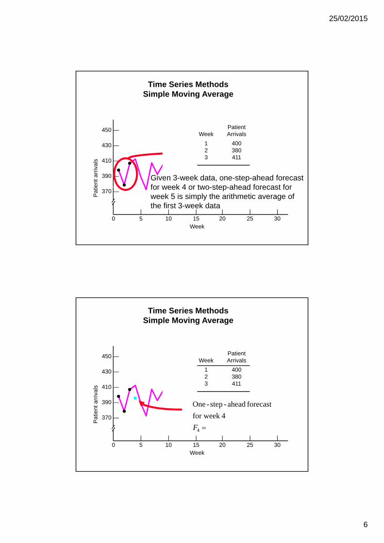
• All these methods will be illustrated with the following example: Suppose that a hospital would like to forecast the number of patients arrival from the following historical p gdata:Week Patients Arrival

1 4002 3803 4114 415

• Note: Although week 4 data is given, some methods require that forecast for period 4 is first computed before computing forecast for period 5.

web4.uwindsor.ca/users/b/.../73.../Lecture_5_Forecasting_f04_331.ppt

Time Series MethodsSimple Moving Average

450

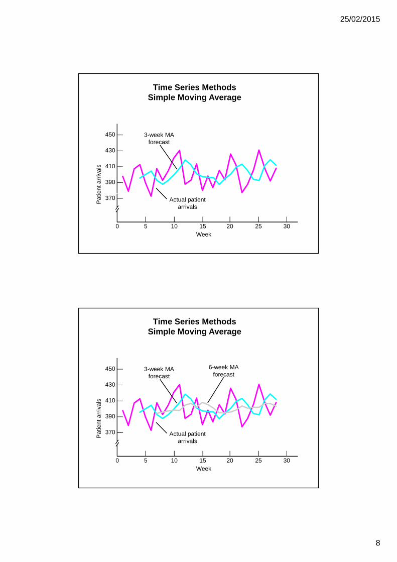
A moving average of order N is simply the arithmetic average of the most recent Nobservations For 3 week moving averages N=3;450 —

430 —

410 —

390 —

ent a

rriva

ls

observations. For 3-week moving averages N=3; for 6-week moving averages N=6; etc.

Week

370 —

Pat

i

| | | | | |0 5 10 15 20 25 30

Actual patientarrivals

25/02/2015

6

450 Patient


450 —

430 —

410 —

390 —

ent a

rriva

ls

PatientWeek Arrivals

1 4002 3803 411

Given 3-week data, one-step-ahead forecast for week 4 or two step ahead forecast for370 —

Pat

i

Week

| | | | | |0 5 10 15 20 25 30

for week 4 or two-step-ahead forecast for week 5 is simply the arithmetic average of the first 3-week data

450 Patient


4f kforecast ahead-step-One

450 —

430 —

410 —

390 —

ent a

rriva

ls

at e tWeek Arrivals

1 4002 3803 411

=4F4for week 370 —

Pat

i

Week

| | | | | |0 5 10 15 20 25 30

25/02/2015

7

450


Patient450 —

430 —

410 —

390 —

ent a

rriva

ls

PatientWeek Arrivals

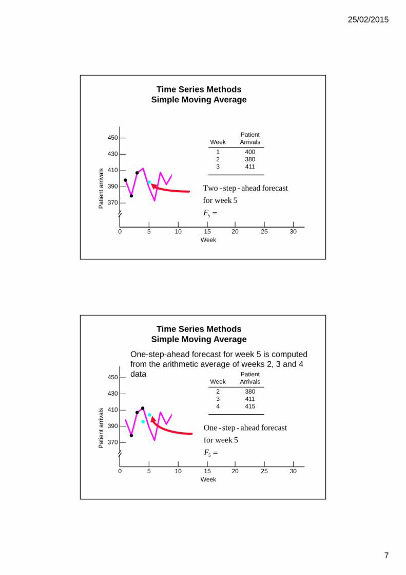
1 4002 3803 411

5f kforecast ahead-step-Two

370 —

Pat

i

| | | | | |0 5 10 15 20 25 30

Week

5for week

=5F

450 Patient


One-step-ahead forecast for week 5 is computed from the arithmetic average of weeks 2, 3 and 4 data450 —

430 —

410 —

390 —

ent a

rriva

ls

at e tWeek Arrivals

2 3803 4114 415

5f kforecast ahead-step-One

data

370 —

Pat

i

Week

| | | | | |0 5 10 15 20 25 30

5for week

=5F

25/02/2015

8

450 3 k MA


450 —

430 —

410 —

390 —

ent a

rriva

ls

3-week MAforecast

370 —

Pat

i

Week

| | | | | |0 5 10 15 20 25 30


450 3 k MA 6-week MA


450 —

430 —

410 —

390 —

ent a

rriva

ls

3-week MAforecast

6-week MAforecast

Week

370 —

Pat

i

| | | | | |0 5 10 15 20 25 30


25/02/2015

9


Single Moving Average

Ide: data pada suatu periode dipengaruhi oleh data beberapa periode sebelumnyabeberapa periode sebelumnyaCocok untuk pola data konstan/stasionerPrinsip dasar:

Data smoothing pada periode ke‐tmerupakan rata‐rata darim buah data dari data periode ke‐t hingga ke‐(t‐m+1) 1 t

t iS X= ∑Data smoothing pada periode ke‐t berperan sebagai nilaiforecasting pada periode ke‐t+1

Ft = St‐1 dan Fn,h = Sn

1t i

i t mm = − +∑


25/02/2015

10

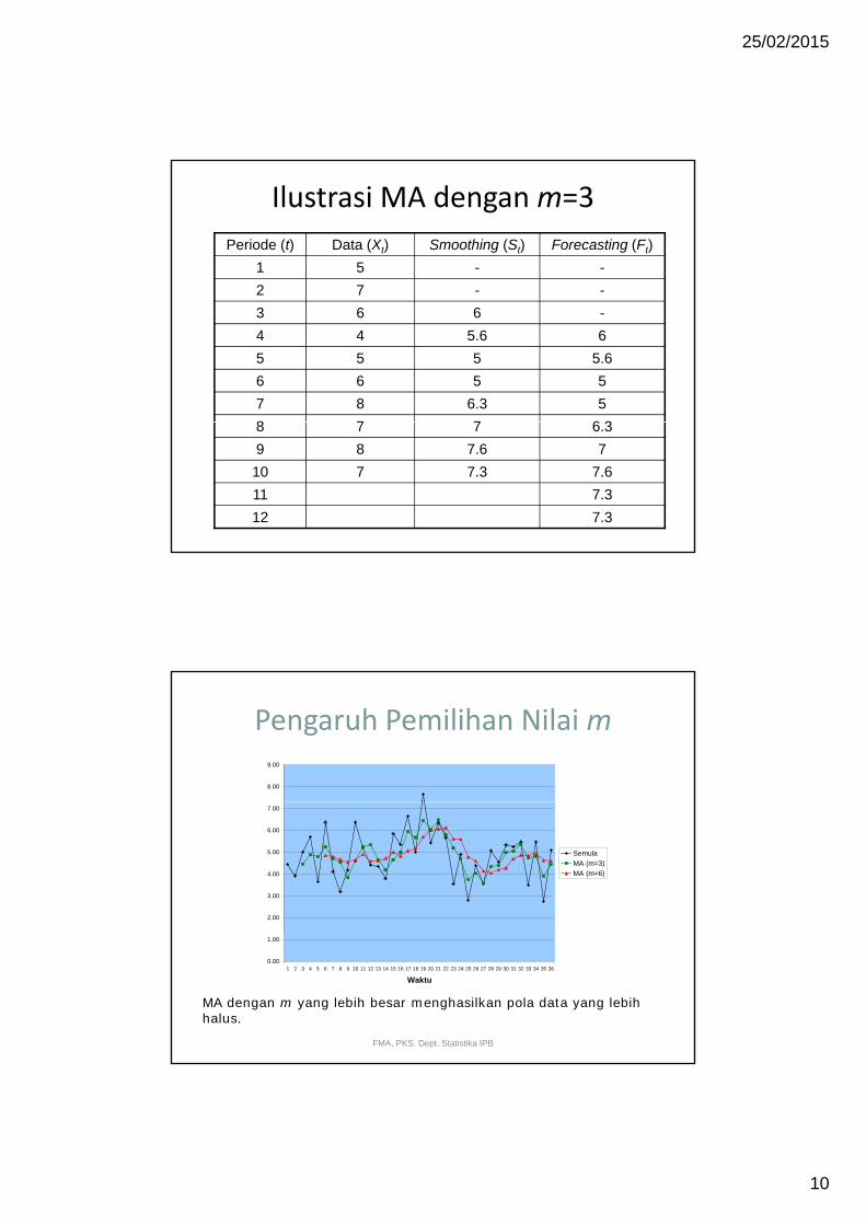
Ilustrasi MA dengan m=3Periode (t) Data (Xt) Smoothing (St) Forecasting (Ft)

1 5 - -2 7 - -2 7 - -3 6 6 -4 4 5.6 65 5 5 5.66 6 5 57 8 6.3 58 7 7 6 38 7 7 6.39 8 7.6 710 7 7.3 7.611 7.312 7.3

Pengaruh Pemilihan Nilai m

8.00

9.00

2.00

3.00

4.00

5.00

6.00

7.00

SemulaMA (m=3)MA (m=6)


0.00

1.00

1 2 3 4 5 6 7 8 9 10 11 12 13 14 15 16 17 18 19 20 21 22 23 24 25 26 27 28 29 30 31 32 33 34 35 36

Waktu

MA dengan m yang lebih besar menghasilkan pola data yang lebih halus.

25/02/2015

11

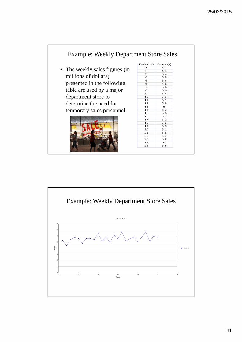
Example: Weekly Department Store Sales

• The weekly sales figures (in millions of dollars)

d i h f ll i

Period (t) Sales (y)1 5,32 4,43 5,44 5,85 5,6presented in the following

table are used by a major department store to determine the need for temporary sales personnel.

5 5,66 4,87 5,68 5,69 5,410 6,511 5,112 5,813 514 6,215 5,616 6,717 5,218 5,519 5,820 5,121 5,822 6,723 5,224 625 5,8


Weekly Sales

8

2

3

4

5

6

7

8

Sale

s

Sales (y)

0

1

2

0 5 10 15 20 25 30

Weeks

25/02/2015

12


• Use a three-week moving average (k=3) for th d t t t l t f t f ththe department store sales to forecast for the week 24 and 26.

• The forecast error is

9.53

8.57.62.53

)(ˆ 21222324 =

++=

++=

yyyy

1.9.56ˆ242424 =−=−= yye


• The forecast for the week 26 is

7.53

2.568.53

ˆ 23242526 =

++=

++=

yyyy

25/02/2015

13

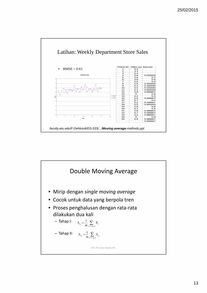
Latihan: Weekly Department Store Sales

Period (t) Sales (y) forecast1 5.3• RMSE = 0.632 4.43 5.44 5.8 5.0333335 5.6 5.26 4.8 5.67 5.6 5.48 5.6 5.3333339 5.4 5.33333310 6.5 5.53333311 5.1 5.83333312 5.8 5.66666713 5 5.814 6.2 5.315 5.6 5.66666716 6.7 5.6

RMSE 0.63Weekly Sales Forecasts

3

4

5

6

7

8

Sale

s Sales (y)

forecast

17 5.2 6.16666718 5.5 5.83333319 5.8 5.820 5.1 5.521 5.8 5.46666722 6.7 5.56666723 5.2 5.86666724 6 5.925 5.8 5.966667

5.666667

0

1

2

3

0 5 10 15 20 25 30

Weeks

faculty.wiu.edu/F-Dehkordi/DS-533/.../Moving-average-methods.ppt

Double Moving Average

• Mirip dengan single moving average• Mirip dengan single moving average• Cocok untuk data yang berpola tren• Proses penghalusan dengan rata‐rata dilakukan dua kali– Tahap I: 1 t

S X= ∑p

– Tahap II:

1,1

t ii t m

S Xm = − +

= ∑

2, 1,1

1 t

t ii t m

S Sm = − +

= ∑


25/02/2015

14

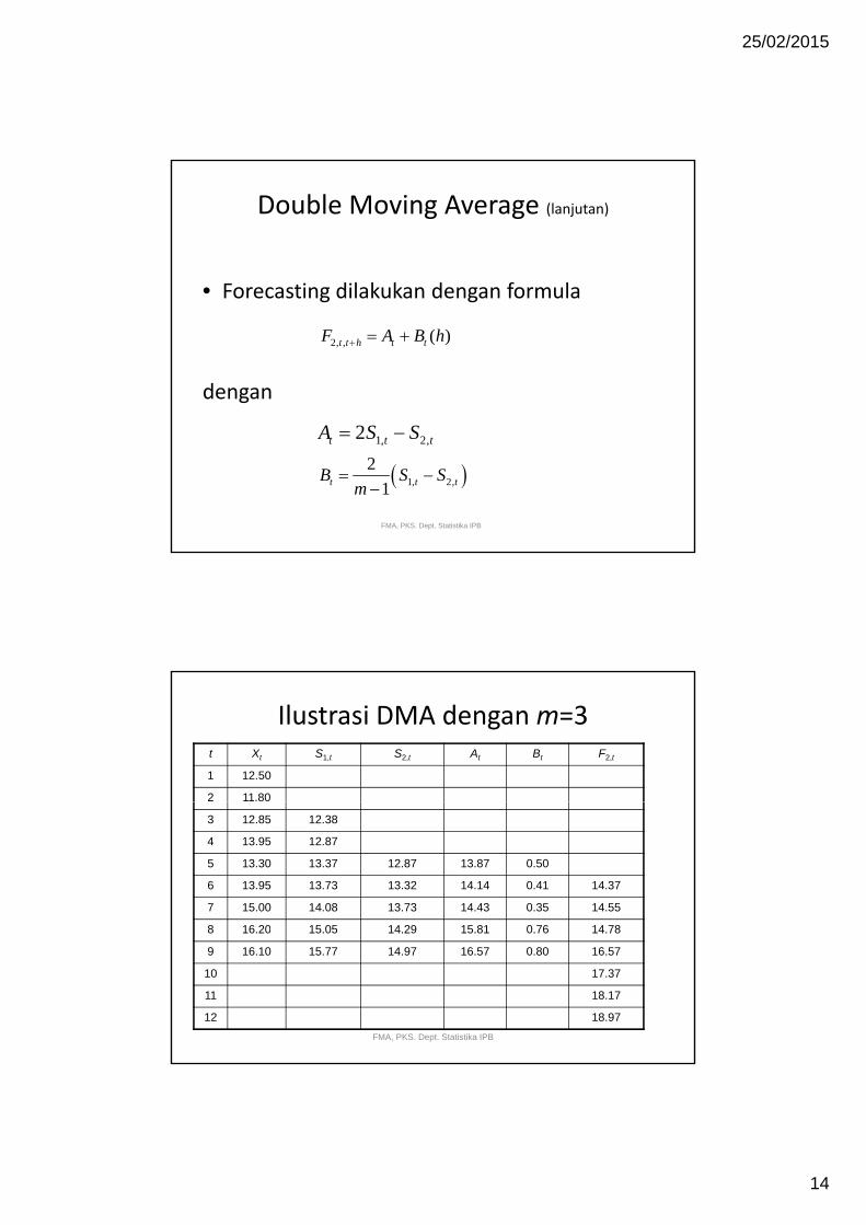
Double Moving Average (lanjutan)

• Forecasting dilakukan dengan formula• Forecasting dilakukan dengan formula

dengan

2, , ( )t t h t tF A B h+ = +

1, 2,2t t tA S S= −


( )1, 2,2

1t t tB S Sm

= −−

Ilustrasi DMA dengan m=3t Xt S1,t S2,t At Bt F2,t

1 12.50

2 11.80

3 12.85 12.38

4 13.95 12.87

5 13.30 13.37 12.87 13.87 0.50

6 13.95 13.73 13.32 14.14 0.41 14.37

7 15.00 14.08 13.73 14.43 0.35 14.55

8 16.20 15.05 14.29 15.81 0.76 14.788 16.20 15.05 14.29 15.81 0.76 14.78

9 16.10 15.77 14.97 16.57 0.80 16.57

10 17.37

11 18.17

12 18.97FMA, PKS. Dept. Statistika IPB

25/02/2015

15

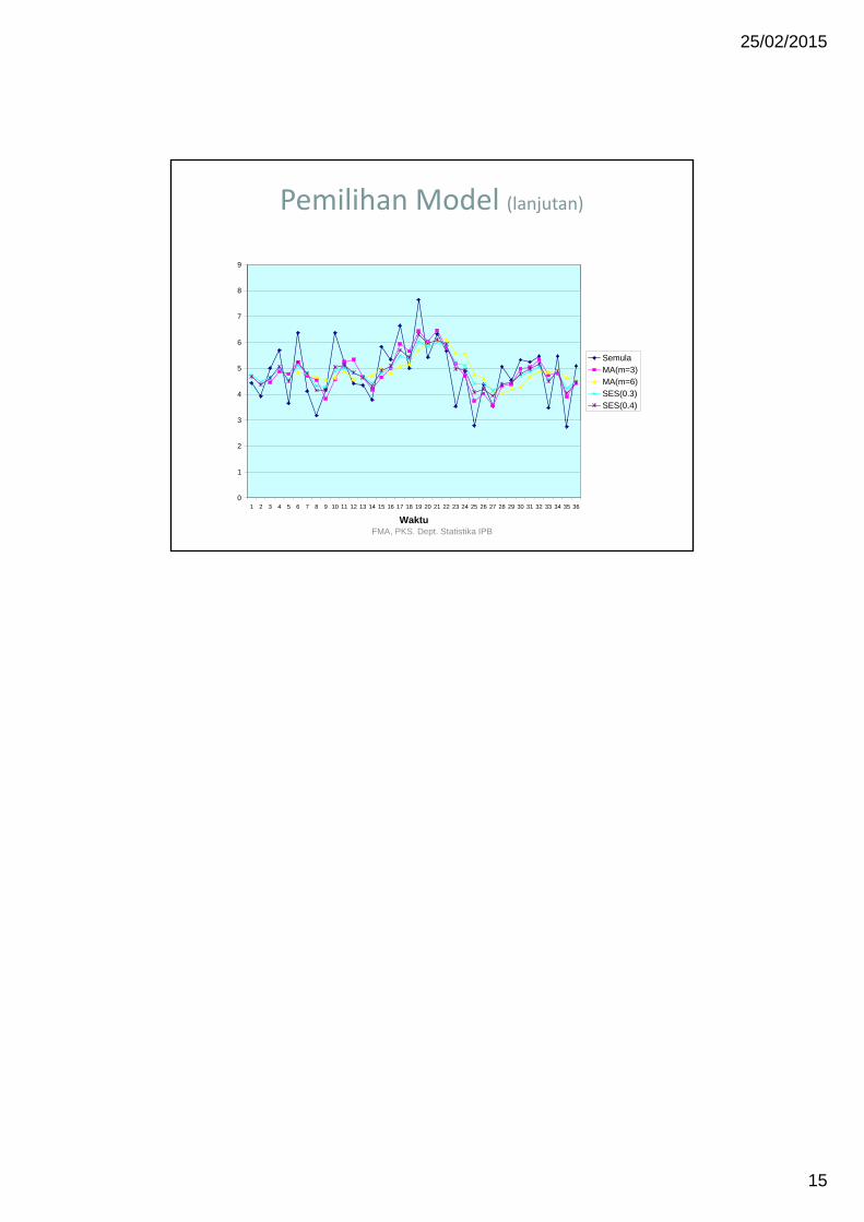
Pemilihan Model (lanjutan)

8

9

3

4

5

6

7

8

SemulaMA(m=3)MA(m=6)SES(0.3)SES(0.4)


0

1

2

3

1 2 3 4 5 6 7 8 9 10 11 12 13 14 15 16 17 18 19 20 21 22 23 24 25 26 27 28 29 30 31 32 33 34 35 36

Waktu

analisis deret waktu - pikasilvianti.staff.ipb.ac.id · ¾harga saham p.t. telkom di bej dari 2...

Documents