1

Pertemuan 04Ukuran Simpangan dan

Variabilitas

Matakuliah : I0134 – Metode Statistika

Tahun : 2007

2

Learning OutcomesPada akhir pertemuan ini, diharapkan mahasiswa akan mampu :

• Mahasiswa akan dapat menghitung ukuran-ukuran variabilitas.

3

Outline Materi

• Range• Inter Quartil Range• Ringkasan Lima Angka• Diagram Kotak Garis• Ukuran Posisi Relative• Varians dan Simpangan Baku

4

Measures of Variability

• A measure along the horizontal axis of the data distribution that describes the spread spread of the distribution from the center.

5

The Range

• The range, R,range, R, of a set of n measurements is the difference between the largest and smallest measurements.

• Example: Example: A botanist records the number of petals on 5 flowers:

5, 12, 6, 8, 14• The range is

R = 14 – 5 = 9.R = 14 – 5 = 9.

•Quick and easy, but only uses 2 of the 5 measurements.•Quick and easy, but only uses 2 of the 5 measurements.

6

The Variance

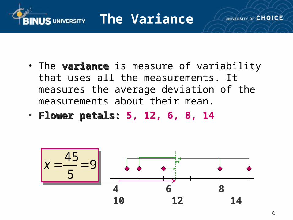
• The variancevariance is measure of variability that uses all the measurements. It measures the average deviation of the measurements about their mean.

• Flower petals:Flower petals: 5, 12, 6, 8, 14

95

45x 9

5

45x

4 6 8 10 12 14

7

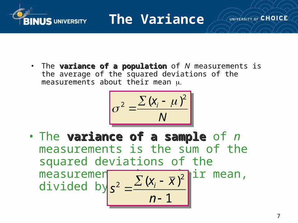
• The variance of a populationvariance of a population of N measurements is the average of the squared deviations of the measurements about their mean

The Variance

• The variance of a samplevariance of a sample of n measurements is the sum of the squared deviations of the measurements about their mean, divided by (n – 1)

N

xi2

2 )(

N

xi2

2 )(

1

)( 22

n

xxs i

1

)( 22

n

xxs i

8

• In calculating the variance, we squared all of the deviations, and in doing so changed the scale of the measurements.

(inch-> square inch)• To return this measure of variability to the original units

of measure, we calculate the standard deviationstandard deviation, the positive square root of the variance.

The Standard Deviation

2

2

:deviation standard Sample

:deviation standard Population

ss

2

2

:deviation standard Sample

:deviation standard Population

ss

9

Two Ways to Calculate the Sample Variance

1

)( 22

n

xxs i

5 -4 16

12 3 9

6 -3 9

8 -1 1

14 5 25

Sum 45 0 60

Use the Definition Formula:ix xxi

2)( xxi

154

60

87.3152 ss

10

Two Ways to Calculate the Sample Variance

1

)( 22

2

nnx

xs

ii

5 25

12 144

6 36

8 64

14 196

Sum 45 465

Use the Calculational Formula:

ix 2ix

154

545

4652

87.3152 ss

11

• The value of s is ALWAYSALWAYS positive.• The larger the value of s2 or s, the larger the

variability of the data set.• Why divide by n –1?Why divide by n –1?

– The sample standard deviation ss is often used to estimate the population standard deviation Dividing by n –1 gives us a better estimate of

Some Notes

AppletApplet

12

Using Measures of Center and Spread: Tchebysheff’s Theorem

Given a number k greater than or equal to 1 and a set of n measurements, at least 1-(1/k2) of the measurement will lie within k standard deviations of the mean.

Given a number k greater than or equal to 1 and a set of n measurements, at least 1-(1/k2) of the measurement will lie within k standard deviations of the mean.

Can be used to describe either samples ( and s) or a population ( and ).Important results: Important results:

If k = 2, at least 1 – 1/22 = 3/4 of the measurements are within 2 standard deviations of the mean.If k = 3, at least 1 – 1/32 = 8/9 of the measurements are within 3 standard deviations of the mean.

x

13

Using Measures of Center and Spread: The Empirical Rule

Given a distribution of measurements that is approximately mound-shaped:

The interval contains approximately 68% of the measurements.

The interval 2 contains approximately 95% of the measurements.

The interval 3 contains approximately 99.7% of the measurements.

Given a distribution of measurements that is approximately mound-shaped:

The interval contains approximately 68% of the measurements.

The interval 2 contains approximately 95% of the measurements.

The interval 3 contains approximately 99.7% of the measurements.

14

Measures of Relative Standing

• How many measurements lie below the measurement of interest? This is measured by the ppth th percentile.percentile.

p-th percentile

(100-p) %x

p %

15

Examples

• 90% of all men (16 and older) earn more than $319 per week.

BUREAU OF LABOR STATISTICS 2002

$319

90%10%

50th Percentile

25th Percentile

75th Percentile

Median

Lower Quartile (Q1) Upper Quartile (Q3)

$319 is the 10th percentile.

$319 is the 10th percentile.

16

• The lower quartile (Qlower quartile (Q11) ) is the value of x which is larger than 25% and less than 75% of the ordered measurements.

• The upper quartile (Qupper quartile (Q33) ) is the value of x which is larger than 75% and less than 25% of the ordered measurements.

• The range of the “middle 50%” of the measurements is the interquartile range, interquartile range,

IQR = IQR = QQ33 – Q – Q11

Quartiles and the IQR

17

Using Measures of Center and Spread: The Box Plot

The Five-Number Summary:

Min Q1 Median Q3 Max

The Five-Number Summary:

Min Q1 Median Q3 Max

•Divides the data into 4 sets containing an equal number of measurements.

•A quick summary of the data distribution.

•Use to form a box plotbox plot to describe the shapeshape of the distribution and to detect outliersoutliers.

18

Constructing a Box Plot

QQ11 mm QQ33

Isolate outliers by calculatingLower fence: Q1-1.5 IQRUpper fence: Q3+1.5 IQR

Measurements beyond the upper or lower fence is are outliers and are marked (*).

*

19

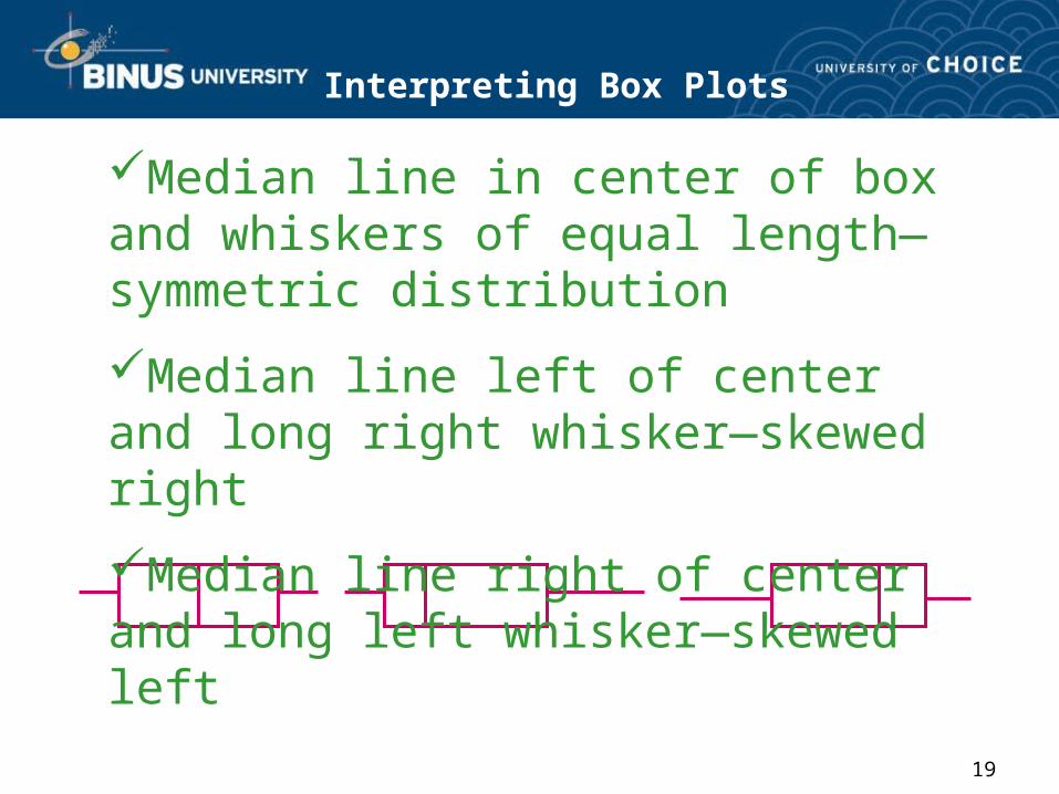
Interpreting Box Plots

Median line in center of box and whiskers of equal length—symmetric distribution

Median line left of center and long right whisker—skewed right

Median line right of center and long left whisker—skewed left

20

Key Concepts

IV. Measures of Relative StandingIV. Measures of Relative Standing1. Sample z-score:2. pth percentile; p% of the measurements are smaller, and (100 p)% are larger.

3. Lower quartile, Q 1; position of Q 1 .25(n 1)

4. Upper quartile, Q 3 ; position of Q 3 .75(n 1)

5. Interquartile range: IQR Q 3 Q 1

V. Box PlotsV. Box Plots

1. Box plots are used for detecting outliers and shapes of distributions.

2. Q 1 and Q 3 form the ends of the box. The median line is in

the interior of the box.

21

Key Concepts

3. Upper and lower fences are used to find outliers.

a. Lower fence: Q 1 1.5(IQR)

b. Outer fences: Q 3 1.5(IQR)

4. Whiskers are connected to the smallest and largest measurements that are not outliers.

5. Skewed distributions usually have a long whisker in the direction of the skewness, and the median line is drawn away from the direction of the skewness.

22

• Selamat Belajar Semoga Sukses.