thumbnail · 2015-03-02 · 1.2.8 chapter 9: phase‐locked loops, 4 1.2.9 chapter 10: power...
TRANSCRIPT
AnAlog And Mixed‐ SignAl electronicS
AnAlog And Mixed‐SignAl electronicS
KArl d StephAnTexas State University San Marcos
Copyright copy 2015 by John Wiley amp Sons Inc All rights reserved
Published by John Wiley amp Sons Inc Hoboken New JerseyPublished simultaneously in Canada
No part of this publication may be reproduced stored in a retrieval system or transmitted in any form or by any means electronic mechanical photocopying recording scanning or otherwise except as permitted under Section 107 or 108 of the 1976 United States Copyright Act without either the prior written permission of the Publisher or authorization through payment of the appropriate per‐copy fee to the Copyright Clearance Center Inc 222 Rosewood Drive Danvers MA 01923 (978) 750‐8400 fax (978) 750‐4470 or on the web at wwwcopyrightcom Requests to the Publisher for permission should be addressed to the Permissions Department John Wiley amp Sons Inc 111 River Street Hoboken NJ 07030 (201) 748‐6011 fax (201) 748‐6008 or online at httpwwwwileycomgopermissions
Limit of LiabilityDisclaimer of Warranty While the publisher and author have used their best efforts in preparing this book they make no representations or warranties with respect to the accuracy or completeness of the contents of this book and specifically disclaim any implied warranties of merchantability or fitness for a particular purpose No warranty may be created or extended by sales representatives or written sales materials The advice and strategies contained herein may not be suitable for your situation You should consult with a professional where appropriate Neither the publisher nor author shall be liable for any loss of profit or any other commercial damages including but not limited to special incidental consequential or other damages
For general information on our other products and services or for technical support please contact our Customer Care Department within the United States at (800) 762‐2974 outside the United States at (317) 572‐3993 or fax (317) 572‐4002
Wiley also publishes its books in a variety of electronic formats Some content that appears in print may not be available in electronic formats For more information about Wiley products visit our web site at wwwwileycom
Library of Congress Cataloging‐in‐Publication Data
Stephan Karl David 1953ndash Analog and mixed-signal electronics Karl D Stephan pages cm Includes bibliographical references and index ISBN 978-1-118-78266-8 (cloth)1 Electronic circuits 2 Mixed signal circuits I Title TK7867S84 2015 6213815ndashdc23
2014050119
Set in 1012pt Times by SPi Publisher Services Pondicherry India
Printed in the United States of America
10 9 8 7 6 5 4 3 2 1
1 2015
contentS
Preface xiAcknowledgments xiiiAbout the companion Website xv
1 Introduction to Analog and Mixed-Signal electronics 1
11 Introduction 112 Organization of the Book 3
121 Chapter 2 Basics of Electronic Components and Devices 3122 Chapter 3 Linear System Analysis 3123 Chapter 4 Nonlinearities in Analog Electronics 3124 Chapter 5 Op Amp Circuits in Analog Electronics 4125 Chapter 6 The High‐Gain Analog Filter Amplifier 4126 Chapter 7 Waveform Generation 4127 Chapter 8 Analog‐to‐Digital and Digital‐to‐Analog Conversion 4128 Chapter 9 Phase‐Locked Loops 4129 Chapter 10 Power Electronics 51210 Chapter 11 High‐Frequency (Radio‐Frequency) Electronics 51211 Chapter 12 Electromagnetic Compatibility 6
Bibliography 6Problems 6
2 Basics of electronic components and Devices 8
21 Introduction 822 Passive Devices 9
221 Resistors 9
vi CONTENTS
222 Capacitors 11223 Inductors 12224 Connectors 13225 Antennas 14
23 Active Devices 15231 Diodes 15232 Field‐Effect Transistors 17233 BJTs 22234 Power Devices 24
Bibliography 29Problems 30
3 Linear Systems Analysis 33
31 Basics of Linear Systems 33311 Two-Terminal Component Models 34312 Two‐Port Matrix Analysis 42
32 Noise and Linear Systems 48321 Sources of Noise 49322 Noise in Designs 53
Bibliography 56Problems 56Project Problem Measurement of Inductor Characteristics 59Equipment and Supplies 59Description 59
4 nonlinearities in Analog electronics 62
41 Why All Amplifiers Are Nonlinear 6242 Effects of Small Nonlinearity 63
421 Second‐Order Nonlinearity 63422 Third‐Order Nonlinearity 67
43 Large‐Scale Nonlinearity Clipping 6944 The Big Picture Dynamic Range 74Bibliography 76Problems 76
5 op Amp circuits in Analog electronics 78
51 Introduction 7852 The Modern Op Amp 80
521 Ideal Equivalent‐Circuit Model 80522 Internal Block Diagram of Typical Op Amp 81523 Op Amp Characteristics 85
53 Analog Circuits Using Op Amps 88531 Linear Op Amp Circuits 92532 Nonlinear Op Amp Circuits 105
CONTENTS vii
Bibliography 115Problems 115
6 the High‐Gain Analog Filter Amplifier 124
61 Applications of High‐Gain Filter Amplifiers 124611 Audio‐Frequency Applications 125612 Sensor Applications 126
62 Issues in High‐Gain Amplifier Design 130621 Dynamic‐Range Problems 130622 Oscillation Problems 131
63 Poles Zeroes Transfer Functions and All That 13464 Passive Analog Filters 137
641 One‐Pole Lowpass Filter 137642 One‐Pole One‐Zero Highpass Filter 141643 Complex‐Pole Bandpass Filter 143644 Bandstop Filters 149
65 Active Analog Filters 149651 SallenndashKey Lowpass Filter with Butterworth Response 150652 Biquad Filter with Lowpass Bandpass or Highpass Response 158653 Switched‐Capacitor Filters 162
66 Design Example Electric Guitar Preamp 164Bibliography 169Problems 169
7 Waveform Generation 175
71 Introduction 17572 ldquoLinearrdquo Sine‐Wave Oscillators and Stability Analysis 176
721 Stable and Unstable Circuits An Example 176722 Poles and Stability 180723 Nyquist Stability Criterion 181724 The Barkhausen Criterion 186725 Noise in Oscillators 189
73 Types of Feedback‐Loop Quasilinear Oscillators 193731 RndashC Oscillators 195732 Quartz‐Crystal Resonators and Oscillators 198733 MEMS Resonators and Oscillators 202
74 Types of Two‐State or Relaxation Oscillators 204741 Astable Multivibrator 205742 555 Timer 207
75 Design Aid Single‐Frequency SeriesndashParallel and ParallelndashSeries Conversion Formulas 209
76 Design Example BJT Quartz‐Crystal Oscillator 211Bibliography 219Problems 219
viii CONTENTS
8 Analog‐to‐Digital and Digital‐to‐Analog conversion 225
81 Introduction 22582 Analog and Digital Signals 226
821 Analog Signals and Measurements 226822 Accuracy Precision and Resolution 227823 Digital Signals and Concepts The Sampling Theorem 230824 Signal Measurements and Quantum Limits 234
83 Basics of Analog‐to‐Digital Conversion 235831 Quantization Error 235832 Output Filtering and Oversampling 237833 Resolution and Speed of ADCs 239
84 Examples of ADC Circuits 242841 Flash Converter 242842 Successive‐Approximation Converter 244843 Delta‐Sigma ADC 245844 Dual‐Slope Integration ADC 250845 Other ADC Approaches 252
85 Examples of DAC Circuits 253851 Rndash2R Ladder DAC 255852 Switched‐Capacitor DAC 256853 One‐Bit DAC 258
86 System‐Level ADC and DAC Operations 259Bibliography 262Problems 262
9 Phase-Locked Loops 269
91 Introduction 26992 Basics of PLLs 27093 Control Theory for PLLs 271
931 First‐Order PLL 273932 Second‐Order PLL 274
94 The CD4046B PLL IC 280941 Phase Detector 1 Exclusive‐OR 280942 Phase Detector 2 Charge Pump 282943 VCO Circuit 285
95 Loop Locking Tuning and Related Issues 28696 PLLs in Frequency Synthesizers 28897 Design Example Using CD4046B PLL IC 289Bibliography 294Problems 294
10 Power electronics 298
101 Introduction 298102 Applications of Power Electronics 300
CONTENTS ix
103 Power Supplies 3001031 Power‐Supply Characteristics and Definitions 3001032 Primary Power Sources 3031033 AC‐to‐DC Conversion in Power Supplies 3061034 Linear Voltage Regulators for Power Supplies 3091035 Switching Power Supplies and Regulators 318
104 Power Amplifiers 3371041 Class A Power Amplifier 3381042 Class B Power Amplifier 3461043 Class AB Power Amplifier 3471044 Class D Power Amplifier 355
105 Devices for Power Electronics Speed and Switching Efficiency 3601051 BJTs 3611052 Power FETs 3611053 IGBTs 3611054 Thyristors 3621055 Vacuum Tubes 362
Bibliography 363Problems 363
11 High‐Frequency (RF) electronics 370
111 Circuits at Radio Frequencies 370112 RF Ranges and Uses 372113 Special Characteristics of RF Circuits 375114 RF Transmission Lines Filters and Impedance‐Matching
Circuits 3761141 RF Transmission Lines 3761142 Filters for Radio‐Frequency Interference
Prevention 3851143 Transmitter and Receiver Filters 3871144 Impedance‐Matching Circuits 389
115 RF Amplifiers 4001151 RF Amplifiers for Transmitters 4001152 RF Amplifiers for Receivers 406
116 Other RF Circuits and Systems 4161161 Mixers 4171162 Phase Shifters and Modulators 4201163 RF Switches 4231164 Oscillators and Multipliers 4231165 Transducers for Photonics and Other Applications 4261166 Antennas 428
117 RF Design Tools 433Bibliography 435Problems 435
x CONTENTS
12 electromagnetic compatibility 446
121 What is Electromagnetic Compatibility 446122 Types of EMI Problems 448
1221 Communications EMI 4481222 Noncommunications EMI 453
123 Modes of EMI Transfer 4541231 Conduction 4541232 Electric Fields (Capacitive EMI) 4561233 Magnetic Fields (Inductive EMI) 4581234 Electromagnetic Fields (Radiation EMI) 461
124 Ways to Reduce EMI 4651241 Bypassing and Filtering 4651242 Grounding 4701243 Shielding 474
125 Designing with EMI and EMC in Mind 4791251 EMC Regulators and Regulations 4791252 Including EMC in Designs 479
Bibliography 481Problems 481
Appendix test equipment for Analog and Mixed‐Signal electronics 489
A1 Introduction 489A2 Laboratory Power Supplies 490A3 Digital Volt‐Ohm‐Milliammeters 492A4 Function Generators 494A5 Oscilloscopes 496A6 Arbitrary Waveform Generators 499A7 Other Types of Analog and Mixed‐Signal Test Equipment 500
A71 Spectrum Analyzers 500A72 Logic Analyzers 501A73 Network Analyzers 501
Index 503
Preface
All but the simplest electronic devices now feature embedded processors and soft-ware development represents the bulk of what many electrical engineers do So some would question the need for a new book on analog and mixed‐signal elec-tronics Surely everything about analog electronics has been known for decades and can be found in old textbooks so what need is there for a new one
In teaching a course on analog and mixed‐signal design for the past few years I have found that as digital and software design has taken over a larger part of the electrical engineering curriculum some important matters relating to analog elec-tronics have fallen into the cracks so to speak Problems as simple as wiring up a dual‐output power supply for an operational amplifier circuit prove daunting to some students whose main engineering tool up to that point has been a computer While all undergraduate electrical engineering students master the basics of linear circuits and systems these subjects are often taught in an abstract isolated fashion that gives no clue as to how the concepts taught can be used to make something worth building and selling which is what engineering is all about
This book is intended to be a practical guide to analog and mixed‐signal elec-tronics with an emphasis on design problems and applications Many examples are included of actual circuit designs developed to meet specific requirements and sev-eral of these have been lab‐tested with experimental results included in the text While advances in analog electronics have not occurred as rapidly as they have in digital systems and software analog systems have found new uses in concert with digital systems leading to the prominence of mixed‐signal systems in many technologies today The modern electrical engineer should be able to address a given design problem with the optimum mix of digital analog and software approaches to get the job done efficiently economically and reliably While most of a systemrsquos
xii PrefAce
functionality may depend on software none of it can get off the ground without power and power supplies are largely still an analog domain
Beginning with reviews of electronic components and linear systems theory this book covers topics such as noise op amps analog filters oscillators conversion between analog and digital domains power electronics and high‐frequency design It closes with a chapter on a subject that is rarely addressed in the undergraduate cur-riculum electromagnetic compatibility Problems having to do with electromagnetic compatibility and electromagnetic interference happen all the time however and can be very difficult to diagnose and fix which is why methods to detect and diagnose such problems are included Although familiarity with standard electrical engi-neering concepts such as complex numbers and Laplace transforms is assumed in parts of the text other parts can be used by those without a calculus or electrical engineering background technicians hobbyists and others interested in analog and mixed‐signal electronics but who are not members of the electrical engineering pro-fession references for further study and a set of problems are provided at the end of each chapter as well as an appendix describing test equipment useful for analog and mixed‐signal work
San Marcos TX Karl D StephanJuly 3 2014
Acknowledgments
ldquoNo man is an island Entire of itselfrdquo as John Donnersquos poem says and this book is my work only in the sense that I am the medium through which it passes Many edu-cators mentors and friends contributed to the knowledge it represents Among these I should mention first the late R David Middlebrook (1929ndash2010) whose electronics course I took as a Caltech undergraduate in the 1970s Professor Middlebrook never met an analog circuit he couldnrsquot analyze with nothing more than paper pencil and a slide rule and his disciplined and insightful approach to analog circuit analysis is an ideal that I am sure I fall short of I can only hope that some of the clarity and depth with which he taught shows through in this text In my 16 years at the University of Massachusetts Amherst I shared teaching responsibilities with my colleagues and friends Robert W Jackson and K Sigfrid Yngvesson Bob Jackson in particular was never the one to let a mathematical or technical ambiguity slip by and I thank him for the quality check he performed on any lecture material we presented jointly A David Wunsch for many years a professor at the University of Massachusetts Lowell reviewed a draft of Chapter 7 and made helpful suggestions for which I am grateful The course entitled ldquoAnalog and Mixed‐Signal Designrdquo was developed at my present institution Texas State University to form part of a new Electrical Engineering program initiated in 2008 The founding Director of the School of Engineering Harold Stern was kind enough to give me a free hand in developing a lab‐based course which has an unconventional structure consisting of four or five multi‐week projects interspersed with lectures I thank him for creating a congenial teaching environment that helped me to develop the material that forms the basis of this text I also thank historian of science Renate Tobies for providing information on Heinrich Barkhausen that is not generally available in English
xiv ACKNoWLEDgMENTS
Finally I express my appreciation and gratitude to my wife Pamela whose artistic skills provided the templates for most of the illustrations Together we can say ldquoBe thankful unto him and bless his name For the Lord is good his mercy is everlasting and his truth endureth to all generationsrdquo
This book is accompanied by a companion websitehttpwileycomgoanalogmixedsignalelectronics
The website includes
bull Solutions Manual available to Instructors
ABoUt tHe comPAnIon weBsIte
Analog and Mixed-Signal Electronics First Edition Karl D Stephan copy 2015 John Wiley amp Sons Inc Published 2015 by John Wiley amp Sons Inc Companion Website httpwileycomgoanalogmixedsignalelectronics
1IntroductIon to AnAlog And MIxed-SIgnAl electronIcS
11 IntroductIon
ldquoIn the beginning there were only analog electronics and vacuum tubes and huge heavy hot equipment that did hardly anything Then came the digitalmdashenabled by integrated circuits and the rapid progress in computers and softwaremdashand electronics became smaller lighter cheaper faster and just better all around all because it was digitalrdquo Thatrsquos the gist of a sort of urban legend that has grown up about the nature of analog electronics and mixed-signal electronics which means simply electronics that has both analog and digital circuitry in it
Like most legends this one has some truth to it Most electronic systems ever since the time that there was anything around to apply the word ldquoelectronicsrdquo to were analog in nature for most of the twentieth century In electronics an analog signal is a voltage or current whose value is proportional to (an analog of) some physical quantity such as sound pressure light intensity or even an abstract numerical value in an analog computer digital signals by contrast ideally take on only one of two values or ranges of values and by doing so represent the discrete binary ones and zeros that form the language of digital computers To give you an idea of how things used to be done with purely analog systems Figure 11 shows on the left a two-channel vacuum-tube audio amplifier that can produce about 70 W per channel
The vacuum-tube amplifier measures 30 cm times 43 cm times 20 cm and weighs 172 kg (38 lb) and was state-of-the-art technology in about 1955 On its right is a solid-state class D amplifier designed in 2008 that can produce about the same amount of
2 InTrODucTIOn TO AnALOg AnD MIxeD-SIgnAL eLecTrOnIcS
output power It is a mixed-signal (analog and digital) design It measures only 15 cm times 10 cm times 4 cm and weighs only 033 kg not including the power supply which is of comparable size and weight The newer amplifier uses its power devices as switches and is much more efficient than the vacuum-tube unit which is about 50 times its size and weight So the claim that many analog designs have been made completely obsolete by newer digital and mixed-signal designs is true as far as it goes
Sometimes you will hear defenders of analog technology argue that ldquothe world is essentially analog and so analog electronics will never go away completelyrdquo Again therersquos some truth to that but it depends on your point of view The physics of quantum mechanics tells us that not only are all material objects made of discrete things called atoms but many forms of energy appear as discrete packets called quanta (photons in the case of electromagnetic radiation) So you can make just as good an argument for the case that the whole world is essentially digital not analog because it can be represented as bits of quanta and atoms that are either there or not there at all
The fact of the matter is that while the bulk of todayrsquos electronics technology is implemented by means of digital circuits and powerful software a smaller but essential part of what goes into most electronic devices involves analog circuitry even if the analog part is as simple as a battery for the power supply no one has yet developed a battery that behaves digitally that is one that provides an absolutely constant voltage until it depletes and drops abruptly to zero So even designers of an otherwise totally digital system have to deal with the analog problem of power-supply characteristics
This book is intended for anyone who has an interest in understanding or designing systems involving analog or mixed-signal electronics That includes undergraduates with a basic sophomore-level understanding of electronics as well as more advanced undergraduates graduate students and professionals in engineering science or other fields whose work requires them to learn about or deal with these types of electronic systems The emphasis is practical rather than theoretical although enough
FIgure 11 A comparison Vacuum‐tube audio amplifier (left) using a design circa 1955 and class D amplifier (right) using a design circa 2008
OrgAnIZATIOn OF THe BOOK 3
theory to enable an understanding of the essentials will be presented as needed throughout Many textbooks present electronics concepts in isolation without any indication of how a component or circuit can be used to meet a practical need and we will try to avoid that error in this book Practical applications of the various circuits and systems described will appear as examples as paper or computer-simulation design exercises and as lab projects
12 orgAnIzAtIon oF the Book
The book is divided into three main sections devices and linear systems (chapters 2 and 3) linear and nonlinear analog circuits and applications (chapters 4ndash7) and special topics of analog and mixed-signal design (chapters 8ndash12) A chapter-by-chapter summary follows
121 chapter 2 Basics of electronic components and devices
In this chapter you will learn enough about the various types of two‐ and three‐terminal electronic devices to use them in simple designs This includes rectifier signal and light‐emitting diodes and the various types of three‐terminal devices field‐effect transistors (FeTs) bipolar junction transistors (BJTs) and power devices Despite the bewildering number of different devices available from manufacturers there are usually only a few specifications that you need to know about each type in order to use them safely and efficiently In this chapter we present basic circuit models for each type of device and how to incorporate the essential specifications into the model
122 chapter 3 linear System Analysis
This chapter presents the basics of linear systems how to characterize a ldquoblack boxrdquo circuit as an element in a more complex system how to deal with characteristics such as gain and frequency response and how to define a systemrsquos overall specifications in terms that can be translated into circuit designs The power of linear analysis is that it can deal with complex systems using fairly simple mathematics You also learn about some basic principles of noise sources and their effects on electronic systems
123 chapter 4 nonlinearities in Analog electronics
While linear analysis covers a great deal of analog‐circuit territory nonlinear effects can both cause problems in designs and provide solutions to other design problems noise of various kinds is always present to some degree in any circuit and in the case of high‐gain and high‐sensitivity systems dealing with low‐level signals noise can determine the performance limits of the entire system You will be introduced to the basics of nonlinearities and noise in this chapter and learn ways of dealing with these issues and minimizing problems that may arise from them
4 InTrODucTIOn TO AnALOg AnD MIxeD-SIgnAL eLecTrOnIcS
124 chapter 5 op Amp circuits in Analog electronics
The workhorse of analog electronics is the operational amplifier (ldquoop amprdquo for short) Originally developed for use in World War II era analog computers in integrated‐circuit form the op amp now plays essential roles in most analog elec-tronics systems of any complexity This chapter describes op amps in a simplified ideal form and outlines the more complex characteristics shown by actual op amps Basic op amp circuits and their uses make up the remainder of the chapter
125 chapter 6 the high‐gain Analog Filter Amplifier
High‐gain amplifiers bring with them unique problems and capabilities so we dedicated an entire chapter to a discussion of the special challenges and techniques needed to develop a good high‐gain amplifier design We also introduce the basics of analog filters in this section and apply them to the design of a practical circuit a guitar preamp
126 chapter 7 Waveform generation
While many electronic systems simply sense or detect signals from the environment other systems produce or generate signals on their own This chapter describes circuits that generate periodic signals collectively termed oscillators as well as other signal‐generation devices Because oscillators that produce a stable frequency output are the heart of all digital clock systems you will also find information on the basics of stabilized oscillators and the means used to stabilize them quartz crystals and more recently microelectromechanical system (MeMS) resonators
127 chapter 8 Analog‐to‐digital and digital‐to‐Analog conversion
Most new electronic designs of any complexity include a microprocessor or equivalent that does the heavy lifting in terms of functionality But many times it is necessary to take analog inputs from various sensors (eg photodiodes ultrasonic sensors proximity detectors) and transform their outputs into a digital format suitable for feeding to the digital microprocessor inputs Similarly you may need to take a digital output from the microprocessor and use it to control an analog or high‐power device such as a lamp or a motor All these problems involve interfacing between analog and digital circuitry While no single solution solves all such problems this chapter describes several techniques you can use to create successful reliable connections between analog systems and digital systems
128 chapter 9 Phase‐locked loops
A phase‐locked loop is a circuit that produces an output waveform whose phase is locked or synchronized to the phase of an input signal Phase‐locked loops are used in a variety of applications ranging from wireless links to biomedical equipment
OrgAnIZATIOn OF THe BOOK 5
This chapter presents the control theory needed for a basic understanding of phase‐locked loops and gives several design examples
129 chapter 10 Power electronics
Most ldquogarden‐varietyrdquo electronic components and systems can control electrical power ranging from less than a microwatt up to a few milliwatts without any special techniques But if you wish to power equipment or devices that need more than 1 W or so you will have to deal with power electronics Audio amplifiers lighting controls and motor controls (including those in increasingly popular electric or hybrid automobiles) all use power electronics Special devices and cir-cuits have been developed to deal with the problems that come when large amounts of electrical power must be produced in a controlled way Because no system is 100 efficient some of the primary input power must be dissipated as heat and as the power delivered rises so does the amount of waste heat that must be gotten rid of somehow in order to keep the power devices from overheating and failing This chapter will introduce you to some basics of power electronics including issues of heat dissipation efficiency calculations and circuit techniques suited for power‐electronics applications Besides conventional linear power‐control circuits the availability of fast switching devices such as insulated‐gate bipolar transis-tors (IgBts) and power FetS means that switch‐mode power systems (those that use active devices as onndashoff switches rather than linear amplifiers) are an increasingly popular way to implement power‐control circuits that have much higher efficiency than their linear‐circuit relatives For this reason we include material on switch‐mode class d amplifiers and switching power supplies in this chapter as well
1210 chapter 11 high‐Frequency (radio‐Frequency) electronics
As long as no signal in a system has a significant frequency component above 20 kHz or so which is the limit of human hearing no special design techniques are needed for most analog circuits However depending on what you are trying to do at frequencies in the MHz range the capacitance of devices cables and simply the cir-cuit wiring itself becomes increasingly significant Above a few MHz the small amount of inductance that short lengths of wire or circuit‐board traces show can also begin to affect the behavior of a circuit At radio frequencies which start at about 1 MHz and extend up to the gHz range a wire is not simply a wire It often must be treated as a transmission line having characteristic values of distributed inductance and capacitance per unit length and sometimes it can even act as an antenna radi-ating some of the power transmitted along it into space
The set of design approaches that deal with these types of high‐frequency prob-lems are known as high‐frequency design or radio-frequency (rF) design This chapter will introduce you to the basics of the field transmission lines filters impedance‐matching circuits and rF circuit techniques such as tuned amplifiers
6 InTrODucTIOn TO AnALOg AnD MIxeD-SIgnAL eLecTrOnIcS
1211 chapter 12 electromagnetic compatibility
electromagnetic compatibility electromagnetic interference and rF interference are usually referred to just by their respective initials eMc eMI and rFI These phrases all refer to various problems that can arise when electromagnetic fields (electric magnetic or a combination) produced by a circuit disturb (or couple to) another circuit usually with undesirable consequences Of course every time you use a mobile tele-phone you employ rF coupling between the phone and the cell‐tower base station that achieves the desirable purpose of making a phone call But the same radio waves that are used in wireless and mobile equipment can also interfere with the proper operation of other electronic systems that are not necessarily designed to receive them While reading this chapter will not make you an eMceMI expert you will learn the basics of how these problems occur and some simple ways to alleviate or avoid them entirely
Following the chapters above is an appendix containing useful information on measurement equipment for analog and mixed‐signal design
each chapter is followed by a set of problems that range from simple applications of concepts developed in the chapter to open‐ended design problems and lab projects While paper designs and simulations using software such as national Instrumentsrsquo Multisimtrade are necessary steps in circuit design the ultimate test of any design is building it This is why we have included many lab‐based projects and encourage both students and instruc-tors to avail themselves of the opportunity of building circuits and trying them out In this field as in many others there is no substitute for hands‐on experience
BIBlIogrAPhy
Analog Devices wwwanalogcom This website of a well‐known analog Ic manufacturer features an electronic periodical called ldquoAnalog Dialoguerdquo as well as numerous datasheets and application notes about a wide variety of analog circuits Ics and applications
crecraft D I and S gergely Analog Electronics Circuits Systems and Signal Processing Oxford uK Butterworth‐Heinemann 2002
Hickman Ian Analog Electronics Second edition Oxford uK newnes 1999
Horowitz P and W Hill The Art of Electronics cambridge uK cambridge university Press 1989
ProBleMS
11 Maximum output power for different waveforms One fundamental limitation of all linear amplifiers is the fact that every amplifier has a maximum voltage output limit it is capable of supplying For example an op amp with a dual power supply of plusmn15 V cannot produce a signal whose voltage exceeds about 25 V peak to peak (V
pp) Assuming that such an amplifier drives a 10‐kΩ load
resistor connected between the output and ground calculate the maximum output power delivered to the load if
PrOBLeMS 7
(a) the 25‐V (peak‐to‐peak) waveform is a pure sine wave (no distortion) and
(b) the 25‐V (peak‐to‐peak) waveform is an ideal square wave (50 duty cycle) (The duty cycle of a pulse is the percentage of the period during which the pulse is high)
12 Efficiency and heat sink limitations Suppose you are using a power device with a heat sink (a mechanical structure designed to dissipate heat into the surround-ing air) and the heat sink can handle up to P
HeAT = 20 W of thermal power (in the
form of heat) before the device becomes dangerously hot above 150degc The power efficiency η of a device is defined as
P
POUT
IN
(11)
and the dissipated thermal power PHeAT
= PIn
minusPOuT
calculate the maximum output power P
OuT that can be obtained from this device‐and‐heat sink
combination if the power efficiency of the device is(a) η = 25 (b) η = 75 (c) η = 90 (d) η = 95 comment on why high
efficiency is so important in high‐power devices
13 Size of circuit compared to wavelength One reason high‐frequency designs must use special techniques is that the signals involved take a finite amount of time to travel through the circuit Suppose you are dealing with a sine‐wave signal at a frequency of 900 MHz and the circuit you design is 25 cm long using the wavelengthndashfrequency relationship
c
f (12)
where λ is the wavelength in meters c is the speed of light (3 times 108 m sminus1) and f is the frequency in Hz (= cycles sminus1 dimensions sminus1) express the length of the circuit in terms of wavelengths at 900 MHz Any time a circuit occupies a substantial fraction of a wavelength in size (more than 10 or so) you should consider using high‐frequency design techniques
14 Reactance of short thin wire at high frequencies If a thin wire 1 cm long is suspended at least a few centimeter away from any nearby conductors it will have an equivalent inductance of about 10 nH (10minus9 H) using the inductive reactance formula X
L = 2πfL calculate the reactance of this length of wire at (a) f
1 = 1 MHz
and (b) f2 = 1 gHz (gHz = gigahertz pronounced ldquogig‐a‐hertzrdquo = 109 Hz) This
shows how parts of a circuit you would not normally consider important such as wire leads can begin to play a significant role in the circuit at high frequencies
For further resources for this chapter visit the companion website at httpwileycomgoanalogmixedsignalelectronics
Analog and Mixed-Signal Electronics First Edition Karl D Stephan copy 2015 John Wiley amp Sons Inc Published 2015 by John Wiley amp Sons Inc Companion Website httpwileycomgoanalogmixedsignalelectronics
2Basics of ElEctronic componEnts and dEvicEs
21 introduction
The term electronic component means any identifiable part that goes into an electronic system Examples of components are resistors capacitors and inductors An electronic device in the sense used in this text is a type of component strictly speaking but generally performs a more complex function than a plain component does A component is usually specified by only one component valuemdashfor example the resistance of a resistor But devices especially three‐terminal devices such as transistors often must be characterized by several parameters in order to predict their behavior adequately in an equivalent‐circuit model
To model a circuit means to create a mathematical structure that models or imitates the way the actual circuit will perform when built Modeling a circuit at some level is almost a necessity because building a circuit without first making a reasonably good mathematical estimate of how it will perform is a waste of time and money Before the advent of digital computers most circuit model calculations were performed by hand and many simplifying assumptions were made Currently proprietary circuit simulation software packages such as PSpicetrade or NI Multisimtrade are typically used to model circuits Whether the calculations are done by hand or with software any circuit model is only as good as the equivalent‐circuit models used for the devices and components in it Simulation programs come with many device and component models already built in but the software manufac-turers cannot always keep up with the rapid development of new devices so the
PASSIVE DEVICES 9
device you want to use may not have an exact equivalent model available in the analysis software you are using
Many circuit models work reasonably well with generic device models and those are the kind we will describe in this chapter simple equivalent circuits with parameters that are adjustable to fit the device you are using A generic model is not associated with any particular manufacturerrsquos model number Instead it has adjustable parameters so that it can behave like any of the different specific devices in its class (another word for class is genus hence the term ldquogenericrdquo) Generic models should be used with caution especially in nonlinear or switching circuits But if a reasonably close match to your device cannot be found in the softwarersquos library of customized device models using a generic model is an alternative
Devices are usually classed into two broad categories passive and active devices The dividing line between passive and active devices is fuzzy but generally passive devices are linear and either store or dissipate power By contrast active devices can amplify or generate signals when embedded in the appropriate circuit and provided with the appropriate AC and DC voltages or currents The passive devices we will describe include resistors capacitors inductors connectors and antennas Active devices include diodes and the various types of small‐signal and power transistors
22 passivE dEvicEs
221 resistors
The need for a component to present a known resistance to current flow arose well before the field of electronics began The designers of nineteenth‐century electric generators found that in order to regulate the output voltage of their machines they had to place a resistive element in series with the field winding that produced the magnetic field which allowed the generator to operate This resistive element was eventually named a resistor and sometimes took the form of a long piece of sheet iron bent into a zigzag shape as shown in Figure 21 which is where the modern symbol for resistors originated
While resistors for power‐control applications can dissipate up to several hundred watts or more most resistors used in ordinary electronic circuits are capable of dissipating only 250 mW or less Specialized devices called power resistors will be discussed in the chapter on power electronics
figurE 21 Early type of bent‐sheet‐metal current‐measurement resistor (1896) from whose shape the schematic‐diagram symbol for resistor was derived
10 BASICS oF ElECTroNIC CoMPoNENTS AND DEVICES
Figure 22 illustrates the well‐known color code followed by most resistor manufacturers for both through‐hole style resistors (also called axial‐lead resistors) and surface‐mount resistors Through‐hole components are manufactured with wire leads that emerge from the componentrsquos body and are typically inserted into the holes in a through‐hole type of printed circuit board (pcB) Through‐hole PCBs were the first type of circuit board developed and are still used for some applications
Resistor identication
ColorBlack 0 0 0
111BrownRed 2
3456789 9 9
8 87 76 65 54 43 3
2 2OrangeYellowGreenBlueVioletGreyWhiteGoldSilver
Surface-mount
bull 0 Ω resistors (marked ldquo0rdquo) are used instead of wire links to simplify robotic assemblybull Resistors less than 100Ω use a 0 multiplier to mean ldquotimes 1rdquo so ldquo100rdquo = 10Ω ldquo470rdquo =47Ω
Surface-mount (SMD) resistors use a similar system Resistance is indicated by a 3-digit code like 104 sometimes followed by a letter Rare precision resistorshave 4 digits (3+ multiplier)
1st Band
1st Digit 2nd Digit 3rd Digit (rare) Multiplier
1104
0 4(10 with 4 zeros)= 100 k Ω
2nd Band 3rd Band Multiplier Tolerance
The end with more bands should point left when reading colors
Inexpensive resistorsusually have 4 bandsand looser tolerance
Better resistors usually have 5 bands and narrower tolerance
times 1 Ωtimes 10 Ωtimes 100 Ωtimes 1k Ωtimes 10k Ωtimes 100k Ωtimes 1M Ωtimes 10M Ω
times 1 Ωtimes 01 Ω
+ndash 1+ndash 2
+ndash 5+ndash 25+ndash 1
+ndash 05
+ndash 5+ndash 10
560k Ωwith +ndash 10 tolerance
237 Ωwith +ndash 1 tolerance
GR
N
BL
U
YE
L
GR
Y
RE
D
OR
G
VLT
BR
N
BL
K
figurE 22 resistor color code for through‐hole resistors and marking code for surface‐mount resistors reproduced by permission of Zach Poff httpwwwzachpoffcomdiy‐resourcesresistor‐color‐code‐chart
PASSIVE DEVICES 11
though the components are typically inserted and soldered by automated machinery rather than by hand surface‐mount technology (smt) uses PCBs with no mounting holes for the components Instead the component and device terminals are formed as conductive areas on the body of the part itself and the contact areas are soldered to corresponding areas on the SMT board surface directly without wires Surface‐mount components can be much smaller than through‐hole components because no wires are needed Automated SMT placement machines can locate the parts with great precision allowing them to be more closely spaced than equivalent through‐hole parts Although SMT boards can be assembled by hand for one‐off prototypes the process is very tedious and error-prone
The physical size of a resistor determines the maximum amount of power it can dissipate so do not expect a 1‐mm2 SMT chip resistor to be able to dissipate much more than 100 mW or so without overheating Although values of resistors available on the market range from a few mΩ (milliohm 10minus3 Ω) (for current‐sampling resistors in high‐current‐measurement circuits) to above 1 gΩ (gigaohm 109 Ω) (for converting extremely small currents into measurable voltages) most analog‐circuit designs should use resistors with values between about 1 Ω and 100 kΩ Values much smaller than 1 Ω are likely to be affected by wiring resistance and values above 100 kΩ can show undesirable changes and instability if a circuit is used in a humid environment and a thin film of water forms in parallel with the resistor
222 capacitors
All capacitors are divided into two types nonelectrolytic or ldquodryrdquo capacitors and electrolytic capacitors The two types are different enough to warrant separate discussions
2221 Nonelectrolytic Capacitors A capacitor consists of two conductive plates or coatings separated by a dielectric (insulator) The value of the capacitance shown by the component is directly proportional to the surface area of the dielectric and inversely proportional to the dielectricrsquos thickness So in order to provide the most capacitance in a given space manufacturers try to use the thinnest dielectric possible and make its area as large as possible Besides determining the value of capacitance the thickness of the dielectric affects the rated voltage of the capacitor Every capacitor will eventually undergo destructive breakdown if the total applied voltage (DC plus peak AC) exceeds its rated voltage Many physically small nonelectrolytic capacitors have rated voltages of only 100 V or less The ceramic or plastic dielectric is so thin that voltages in excess of 100 V will cause destructive breakdown leading to a shorted device and possibly system failure
Most capacitor values are marked on the body of the device either directly (eg ldquo1 μFrdquo meaning 1 microfarad 10minus6 F) or in terms of pf (picofarads 10minus12 F) in the same way SMT resistors are marked For example a capacitor marked ldquo103rdquo usually has a value of 10 times 103 or 10000 pF which is equivalent to 10 nF (nanofarads 10minus9 F) Voltage ratings for the smaller capacitors are often not marked and must be determined from the catalog description Nonelectrolytic capacitors are not polarized
12 BASICS oF ElECTroNIC CoMPoNENTS AND DEVICES
and can usually be reversed (terminals exchanged) without affecting the circuit performance adversely in nearly all cases Virtually all capacitors with values less than 1 μF are nonelectrolytic capacitors
2222 Electrolytic Capacitors Most capacitors with values of 1 μF or larger are electrolytic capacitors These capacitors are made by separating two conductive sheets of aluminum or tantalum with a thin moist electrolytic paste and then forming a dielectric layer only a few nm (nanometer 10minus9 m) thick on one of the plates electrolytically Because such a thin dielectric produces a large capacitance per unit area electrolytic capacitors can show extremely large capacitance values (from 1 μF up into the mF (millifarad 10minus3 F) range) in packages of reasonable size However their method of manufacture means that they can withstand their rated voltage only if the proper polarity is observed This means that strictly speaking one should not use an electrolytic capacitor in a circuit where AC only appears across it because half the time the AC waveform will apply the wrong polarity to the capacitor and it may fail prematurely If an electrolytic capacitor is connected backward so that a large DC voltage is applied to it with the wrong polarity the heat generated can vaporize the water inside and cause the capacitor to explode Besides the damage this causes it can be really embarrassing in a lab full of other students if your circuit literally blows up
Specially constructed capacitors called supercapacitors can provide even more capacitance in a given volume than conventional electrolytic capacitors by electrochemical means that lie between the conventional dielectric‐layer structure of electrolytic capacitors and the chemical processes that take place in a battery (electrochemical cell) Supercapacitors can have values in the multifarad range but tend to have low maximum rated voltages and are more costly than electrolytic units of similar ratings
223 inductors
Just as capacitors store energy in an electrostatic field inductors store energy in a magnetic field Because of the physics of magnetic fields most inductors consist of many turns (loops) of insulated wire wound around a central core The core may be hollow (a so‐called air‐core coil) or filled with a material such as iron steel or ferrite (a type of ceramic) that has desirable magnetic properties The use of a magnetic core material allows greater inductance to be obtained in the same physical space
one can always obtain more inductance in a given volume by winding more turns around the core In order to do this in the same space however the wire must be made thinner and thin wire has more resistance per unit length than thick wire does The wirersquos resistance appears in the inductorrsquos equivalent circuit along with the desired property of inductance and too large a resistance makes the inductor less useful for most applications Designers of inductors choose the wire size number of turns and core material to fit a given application taking into consideration such factors as space available and the intended frequency range of operation
In general inductors are used in analog circuits only when necessary because for values above a few microhenries (μH 10minus6 H) these components tend to be bulky

Analog and Mixed-Signal Electronics First Edition Karl D Stephan copy 2015 John Wiley amp Sons Inc Published 2015 by John Wiley amp Sons Inc Companion Website httpwileycomgoanalogmixedsignalelectronics
1IntroductIon to AnAlog And MIxed-SIgnAl electronIcS
11 IntroductIon
ldquoIn the beginning there were only analog electronics and vacuum tubes and huge heavy hot equipment that did hardly anything Then came the digitalmdashenabled by integrated circuits and the rapid progress in computers and softwaremdashand electronics became smaller lighter cheaper faster and just better all around all because it was digitalrdquo Thatrsquos the gist of a sort of urban legend that has grown up about the nature of analog electronics and mixed-signal electronics which means simply electronics that has both analog and digital circuitry in it
Like most legends this one has some truth to it Most electronic systems ever since the time that there was anything around to apply the word ldquoelectronicsrdquo to were analog in nature for most of the twentieth century In electronics an analog signal is a voltage or current whose value is proportional to (an analog of) some physical quantity such as sound pressure light intensity or even an abstract numerical value in an analog computer digital signals by contrast ideally take on only one of two values or ranges of values and by doing so represent the discrete binary ones and zeros that form the language of digital computers To give you an idea of how things used to be done with purely analog systems Figure 11 shows on the left a two-channel vacuum-tube audio amplifier that can produce about 70 W per channel
The vacuum-tube amplifier measures 30 cm times 43 cm times 20 cm and weighs 172 kg (38 lb) and was state-of-the-art technology in about 1955 On its right is a solid-state class D amplifier designed in 2008 that can produce about the same amount of
2 InTrODucTIOn TO AnALOg AnD MIxeD-SIgnAL eLecTrOnIcS
output power It is a mixed-signal (analog and digital) design It measures only 15 cm times 10 cm times 4 cm and weighs only 033 kg not including the power supply which is of comparable size and weight The newer amplifier uses its power devices as switches and is much more efficient than the vacuum-tube unit which is about 50 times its size and weight So the claim that many analog designs have been made completely obsolete by newer digital and mixed-signal designs is true as far as it goes
Sometimes you will hear defenders of analog technology argue that ldquothe world is essentially analog and so analog electronics will never go away completelyrdquo Again therersquos some truth to that but it depends on your point of view The physics of quantum mechanics tells us that not only are all material objects made of discrete things called atoms but many forms of energy appear as discrete packets called quanta (photons in the case of electromagnetic radiation) So you can make just as good an argument for the case that the whole world is essentially digital not analog because it can be represented as bits of quanta and atoms that are either there or not there at all
The fact of the matter is that while the bulk of todayrsquos electronics technology is implemented by means of digital circuits and powerful software a smaller but essential part of what goes into most electronic devices involves analog circuitry even if the analog part is as simple as a battery for the power supply no one has yet developed a battery that behaves digitally that is one that provides an absolutely constant voltage until it depletes and drops abruptly to zero So even designers of an otherwise totally digital system have to deal with the analog problem of power-supply characteristics
This book is intended for anyone who has an interest in understanding or designing systems involving analog or mixed-signal electronics That includes undergraduates with a basic sophomore-level understanding of electronics as well as more advanced undergraduates graduate students and professionals in engineering science or other fields whose work requires them to learn about or deal with these types of electronic systems The emphasis is practical rather than theoretical although enough
FIgure 11 A comparison Vacuum‐tube audio amplifier (left) using a design circa 1955 and class D amplifier (right) using a design circa 2008
OrgAnIZATIOn OF THe BOOK 3
theory to enable an understanding of the essentials will be presented as needed throughout Many textbooks present electronics concepts in isolation without any indication of how a component or circuit can be used to meet a practical need and we will try to avoid that error in this book Practical applications of the various circuits and systems described will appear as examples as paper or computer-simulation design exercises and as lab projects
12 orgAnIzAtIon oF the Book
The book is divided into three main sections devices and linear systems (chapters 2 and 3) linear and nonlinear analog circuits and applications (chapters 4ndash7) and special topics of analog and mixed-signal design (chapters 8ndash12) A chapter-by-chapter summary follows
121 chapter 2 Basics of electronic components and devices
In this chapter you will learn enough about the various types of two‐ and three‐terminal electronic devices to use them in simple designs This includes rectifier signal and light‐emitting diodes and the various types of three‐terminal devices field‐effect transistors (FeTs) bipolar junction transistors (BJTs) and power devices Despite the bewildering number of different devices available from manufacturers there are usually only a few specifications that you need to know about each type in order to use them safely and efficiently In this chapter we present basic circuit models for each type of device and how to incorporate the essential specifications into the model
122 chapter 3 linear System Analysis
This chapter presents the basics of linear systems how to characterize a ldquoblack boxrdquo circuit as an element in a more complex system how to deal with characteristics such as gain and frequency response and how to define a systemrsquos overall specifications in terms that can be translated into circuit designs The power of linear analysis is that it can deal with complex systems using fairly simple mathematics You also learn about some basic principles of noise sources and their effects on electronic systems
123 chapter 4 nonlinearities in Analog electronics
While linear analysis covers a great deal of analog‐circuit territory nonlinear effects can both cause problems in designs and provide solutions to other design problems noise of various kinds is always present to some degree in any circuit and in the case of high‐gain and high‐sensitivity systems dealing with low‐level signals noise can determine the performance limits of the entire system You will be introduced to the basics of nonlinearities and noise in this chapter and learn ways of dealing with these issues and minimizing problems that may arise from them
4 InTrODucTIOn TO AnALOg AnD MIxeD-SIgnAL eLecTrOnIcS
124 chapter 5 op Amp circuits in Analog electronics
The workhorse of analog electronics is the operational amplifier (ldquoop amprdquo for short) Originally developed for use in World War II era analog computers in integrated‐circuit form the op amp now plays essential roles in most analog elec-tronics systems of any complexity This chapter describes op amps in a simplified ideal form and outlines the more complex characteristics shown by actual op amps Basic op amp circuits and their uses make up the remainder of the chapter
125 chapter 6 the high‐gain Analog Filter Amplifier
High‐gain amplifiers bring with them unique problems and capabilities so we dedicated an entire chapter to a discussion of the special challenges and techniques needed to develop a good high‐gain amplifier design We also introduce the basics of analog filters in this section and apply them to the design of a practical circuit a guitar preamp
126 chapter 7 Waveform generation
While many electronic systems simply sense or detect signals from the environment other systems produce or generate signals on their own This chapter describes circuits that generate periodic signals collectively termed oscillators as well as other signal‐generation devices Because oscillators that produce a stable frequency output are the heart of all digital clock systems you will also find information on the basics of stabilized oscillators and the means used to stabilize them quartz crystals and more recently microelectromechanical system (MeMS) resonators
127 chapter 8 Analog‐to‐digital and digital‐to‐Analog conversion
Most new electronic designs of any complexity include a microprocessor or equivalent that does the heavy lifting in terms of functionality But many times it is necessary to take analog inputs from various sensors (eg photodiodes ultrasonic sensors proximity detectors) and transform their outputs into a digital format suitable for feeding to the digital microprocessor inputs Similarly you may need to take a digital output from the microprocessor and use it to control an analog or high‐power device such as a lamp or a motor All these problems involve interfacing between analog and digital circuitry While no single solution solves all such problems this chapter describes several techniques you can use to create successful reliable connections between analog systems and digital systems
128 chapter 9 Phase‐locked loops
A phase‐locked loop is a circuit that produces an output waveform whose phase is locked or synchronized to the phase of an input signal Phase‐locked loops are used in a variety of applications ranging from wireless links to biomedical equipment
OrgAnIZATIOn OF THe BOOK 5
This chapter presents the control theory needed for a basic understanding of phase‐locked loops and gives several design examples
129 chapter 10 Power electronics
Most ldquogarden‐varietyrdquo electronic components and systems can control electrical power ranging from less than a microwatt up to a few milliwatts without any special techniques But if you wish to power equipment or devices that need more than 1 W or so you will have to deal with power electronics Audio amplifiers lighting controls and motor controls (including those in increasingly popular electric or hybrid automobiles) all use power electronics Special devices and cir-cuits have been developed to deal with the problems that come when large amounts of electrical power must be produced in a controlled way Because no system is 100 efficient some of the primary input power must be dissipated as heat and as the power delivered rises so does the amount of waste heat that must be gotten rid of somehow in order to keep the power devices from overheating and failing This chapter will introduce you to some basics of power electronics including issues of heat dissipation efficiency calculations and circuit techniques suited for power‐electronics applications Besides conventional linear power‐control circuits the availability of fast switching devices such as insulated‐gate bipolar transis-tors (IgBts) and power FetS means that switch‐mode power systems (those that use active devices as onndashoff switches rather than linear amplifiers) are an increasingly popular way to implement power‐control circuits that have much higher efficiency than their linear‐circuit relatives For this reason we include material on switch‐mode class d amplifiers and switching power supplies in this chapter as well
1210 chapter 11 high‐Frequency (radio‐Frequency) electronics
As long as no signal in a system has a significant frequency component above 20 kHz or so which is the limit of human hearing no special design techniques are needed for most analog circuits However depending on what you are trying to do at frequencies in the MHz range the capacitance of devices cables and simply the cir-cuit wiring itself becomes increasingly significant Above a few MHz the small amount of inductance that short lengths of wire or circuit‐board traces show can also begin to affect the behavior of a circuit At radio frequencies which start at about 1 MHz and extend up to the gHz range a wire is not simply a wire It often must be treated as a transmission line having characteristic values of distributed inductance and capacitance per unit length and sometimes it can even act as an antenna radi-ating some of the power transmitted along it into space
The set of design approaches that deal with these types of high‐frequency prob-lems are known as high‐frequency design or radio-frequency (rF) design This chapter will introduce you to the basics of the field transmission lines filters impedance‐matching circuits and rF circuit techniques such as tuned amplifiers
6 InTrODucTIOn TO AnALOg AnD MIxeD-SIgnAL eLecTrOnIcS
1211 chapter 12 electromagnetic compatibility
electromagnetic compatibility electromagnetic interference and rF interference are usually referred to just by their respective initials eMc eMI and rFI These phrases all refer to various problems that can arise when electromagnetic fields (electric magnetic or a combination) produced by a circuit disturb (or couple to) another circuit usually with undesirable consequences Of course every time you use a mobile tele-phone you employ rF coupling between the phone and the cell‐tower base station that achieves the desirable purpose of making a phone call But the same radio waves that are used in wireless and mobile equipment can also interfere with the proper operation of other electronic systems that are not necessarily designed to receive them While reading this chapter will not make you an eMceMI expert you will learn the basics of how these problems occur and some simple ways to alleviate or avoid them entirely
Following the chapters above is an appendix containing useful information on measurement equipment for analog and mixed‐signal design
each chapter is followed by a set of problems that range from simple applications of concepts developed in the chapter to open‐ended design problems and lab projects While paper designs and simulations using software such as national Instrumentsrsquo Multisimtrade are necessary steps in circuit design the ultimate test of any design is building it This is why we have included many lab‐based projects and encourage both students and instruc-tors to avail themselves of the opportunity of building circuits and trying them out In this field as in many others there is no substitute for hands‐on experience
BIBlIogrAPhy
Analog Devices wwwanalogcom This website of a well‐known analog Ic manufacturer features an electronic periodical called ldquoAnalog Dialoguerdquo as well as numerous datasheets and application notes about a wide variety of analog circuits Ics and applications
crecraft D I and S gergely Analog Electronics Circuits Systems and Signal Processing Oxford uK Butterworth‐Heinemann 2002
Hickman Ian Analog Electronics Second edition Oxford uK newnes 1999
Horowitz P and W Hill The Art of Electronics cambridge uK cambridge university Press 1989
ProBleMS
11 Maximum output power for different waveforms One fundamental limitation of all linear amplifiers is the fact that every amplifier has a maximum voltage output limit it is capable of supplying For example an op amp with a dual power supply of plusmn15 V cannot produce a signal whose voltage exceeds about 25 V peak to peak (V
pp) Assuming that such an amplifier drives a 10‐kΩ load
resistor connected between the output and ground calculate the maximum output power delivered to the load if
PrOBLeMS 7
(a) the 25‐V (peak‐to‐peak) waveform is a pure sine wave (no distortion) and
(b) the 25‐V (peak‐to‐peak) waveform is an ideal square wave (50 duty cycle) (The duty cycle of a pulse is the percentage of the period during which the pulse is high)
12 Efficiency and heat sink limitations Suppose you are using a power device with a heat sink (a mechanical structure designed to dissipate heat into the surround-ing air) and the heat sink can handle up to P
HeAT = 20 W of thermal power (in the
form of heat) before the device becomes dangerously hot above 150degc The power efficiency η of a device is defined as
P
POUT
IN
(11)
and the dissipated thermal power PHeAT
= PIn
minusPOuT
calculate the maximum output power P
OuT that can be obtained from this device‐and‐heat sink
combination if the power efficiency of the device is(a) η = 25 (b) η = 75 (c) η = 90 (d) η = 95 comment on why high
efficiency is so important in high‐power devices
13 Size of circuit compared to wavelength One reason high‐frequency designs must use special techniques is that the signals involved take a finite amount of time to travel through the circuit Suppose you are dealing with a sine‐wave signal at a frequency of 900 MHz and the circuit you design is 25 cm long using the wavelengthndashfrequency relationship
c
f (12)
where λ is the wavelength in meters c is the speed of light (3 times 108 m sminus1) and f is the frequency in Hz (= cycles sminus1 dimensions sminus1) express the length of the circuit in terms of wavelengths at 900 MHz Any time a circuit occupies a substantial fraction of a wavelength in size (more than 10 or so) you should consider using high‐frequency design techniques
14 Reactance of short thin wire at high frequencies If a thin wire 1 cm long is suspended at least a few centimeter away from any nearby conductors it will have an equivalent inductance of about 10 nH (10minus9 H) using the inductive reactance formula X
L = 2πfL calculate the reactance of this length of wire at (a) f
1 = 1 MHz
and (b) f2 = 1 gHz (gHz = gigahertz pronounced ldquogig‐a‐hertzrdquo = 109 Hz) This
shows how parts of a circuit you would not normally consider important such as wire leads can begin to play a significant role in the circuit at high frequencies
For further resources for this chapter visit the companion website at httpwileycomgoanalogmixedsignalelectronics
Analog and Mixed-Signal Electronics First Edition Karl D Stephan copy 2015 John Wiley amp Sons Inc Published 2015 by John Wiley amp Sons Inc Companion Website httpwileycomgoanalogmixedsignalelectronics
2Basics of ElEctronic componEnts and dEvicEs
21 introduction
The term electronic component means any identifiable part that goes into an electronic system Examples of components are resistors capacitors and inductors An electronic device in the sense used in this text is a type of component strictly speaking but generally performs a more complex function than a plain component does A component is usually specified by only one component valuemdashfor example the resistance of a resistor But devices especially three‐terminal devices such as transistors often must be characterized by several parameters in order to predict their behavior adequately in an equivalent‐circuit model
To model a circuit means to create a mathematical structure that models or imitates the way the actual circuit will perform when built Modeling a circuit at some level is almost a necessity because building a circuit without first making a reasonably good mathematical estimate of how it will perform is a waste of time and money Before the advent of digital computers most circuit model calculations were performed by hand and many simplifying assumptions were made Currently proprietary circuit simulation software packages such as PSpicetrade or NI Multisimtrade are typically used to model circuits Whether the calculations are done by hand or with software any circuit model is only as good as the equivalent‐circuit models used for the devices and components in it Simulation programs come with many device and component models already built in but the software manufac-turers cannot always keep up with the rapid development of new devices so the
PASSIVE DEVICES 9
device you want to use may not have an exact equivalent model available in the analysis software you are using
Many circuit models work reasonably well with generic device models and those are the kind we will describe in this chapter simple equivalent circuits with parameters that are adjustable to fit the device you are using A generic model is not associated with any particular manufacturerrsquos model number Instead it has adjustable parameters so that it can behave like any of the different specific devices in its class (another word for class is genus hence the term ldquogenericrdquo) Generic models should be used with caution especially in nonlinear or switching circuits But if a reasonably close match to your device cannot be found in the softwarersquos library of customized device models using a generic model is an alternative
Devices are usually classed into two broad categories passive and active devices The dividing line between passive and active devices is fuzzy but generally passive devices are linear and either store or dissipate power By contrast active devices can amplify or generate signals when embedded in the appropriate circuit and provided with the appropriate AC and DC voltages or currents The passive devices we will describe include resistors capacitors inductors connectors and antennas Active devices include diodes and the various types of small‐signal and power transistors
22 passivE dEvicEs
221 resistors
The need for a component to present a known resistance to current flow arose well before the field of electronics began The designers of nineteenth‐century electric generators found that in order to regulate the output voltage of their machines they had to place a resistive element in series with the field winding that produced the magnetic field which allowed the generator to operate This resistive element was eventually named a resistor and sometimes took the form of a long piece of sheet iron bent into a zigzag shape as shown in Figure 21 which is where the modern symbol for resistors originated
While resistors for power‐control applications can dissipate up to several hundred watts or more most resistors used in ordinary electronic circuits are capable of dissipating only 250 mW or less Specialized devices called power resistors will be discussed in the chapter on power electronics
figurE 21 Early type of bent‐sheet‐metal current‐measurement resistor (1896) from whose shape the schematic‐diagram symbol for resistor was derived
10 BASICS oF ElECTroNIC CoMPoNENTS AND DEVICES
Figure 22 illustrates the well‐known color code followed by most resistor manufacturers for both through‐hole style resistors (also called axial‐lead resistors) and surface‐mount resistors Through‐hole components are manufactured with wire leads that emerge from the componentrsquos body and are typically inserted into the holes in a through‐hole type of printed circuit board (pcB) Through‐hole PCBs were the first type of circuit board developed and are still used for some applications
Resistor identication
ColorBlack 0 0 0
111BrownRed 2
3456789 9 9
8 87 76 65 54 43 3
2 2OrangeYellowGreenBlueVioletGreyWhiteGoldSilver
Surface-mount
bull 0 Ω resistors (marked ldquo0rdquo) are used instead of wire links to simplify robotic assemblybull Resistors less than 100Ω use a 0 multiplier to mean ldquotimes 1rdquo so ldquo100rdquo = 10Ω ldquo470rdquo =47Ω
Surface-mount (SMD) resistors use a similar system Resistance is indicated by a 3-digit code like 104 sometimes followed by a letter Rare precision resistorshave 4 digits (3+ multiplier)
1st Band
1st Digit 2nd Digit 3rd Digit (rare) Multiplier
1104
0 4(10 with 4 zeros)= 100 k Ω
2nd Band 3rd Band Multiplier Tolerance
The end with more bands should point left when reading colors
Inexpensive resistorsusually have 4 bandsand looser tolerance
Better resistors usually have 5 bands and narrower tolerance
times 1 Ωtimes 10 Ωtimes 100 Ωtimes 1k Ωtimes 10k Ωtimes 100k Ωtimes 1M Ωtimes 10M Ω
times 1 Ωtimes 01 Ω
+ndash 1+ndash 2
+ndash 5+ndash 25+ndash 1
+ndash 05
+ndash 5+ndash 10
560k Ωwith +ndash 10 tolerance
237 Ωwith +ndash 1 tolerance
GR
N
BL
U
YE
L
GR
Y
RE
D
OR
G
VLT
BR
N
BL
K
figurE 22 resistor color code for through‐hole resistors and marking code for surface‐mount resistors reproduced by permission of Zach Poff httpwwwzachpoffcomdiy‐resourcesresistor‐color‐code‐chart
PASSIVE DEVICES 11
though the components are typically inserted and soldered by automated machinery rather than by hand surface‐mount technology (smt) uses PCBs with no mounting holes for the components Instead the component and device terminals are formed as conductive areas on the body of the part itself and the contact areas are soldered to corresponding areas on the SMT board surface directly without wires Surface‐mount components can be much smaller than through‐hole components because no wires are needed Automated SMT placement machines can locate the parts with great precision allowing them to be more closely spaced than equivalent through‐hole parts Although SMT boards can be assembled by hand for one‐off prototypes the process is very tedious and error-prone
The physical size of a resistor determines the maximum amount of power it can dissipate so do not expect a 1‐mm2 SMT chip resistor to be able to dissipate much more than 100 mW or so without overheating Although values of resistors available on the market range from a few mΩ (milliohm 10minus3 Ω) (for current‐sampling resistors in high‐current‐measurement circuits) to above 1 gΩ (gigaohm 109 Ω) (for converting extremely small currents into measurable voltages) most analog‐circuit designs should use resistors with values between about 1 Ω and 100 kΩ Values much smaller than 1 Ω are likely to be affected by wiring resistance and values above 100 kΩ can show undesirable changes and instability if a circuit is used in a humid environment and a thin film of water forms in parallel with the resistor
222 capacitors
All capacitors are divided into two types nonelectrolytic or ldquodryrdquo capacitors and electrolytic capacitors The two types are different enough to warrant separate discussions
2221 Nonelectrolytic Capacitors A capacitor consists of two conductive plates or coatings separated by a dielectric (insulator) The value of the capacitance shown by the component is directly proportional to the surface area of the dielectric and inversely proportional to the dielectricrsquos thickness So in order to provide the most capacitance in a given space manufacturers try to use the thinnest dielectric possible and make its area as large as possible Besides determining the value of capacitance the thickness of the dielectric affects the rated voltage of the capacitor Every capacitor will eventually undergo destructive breakdown if the total applied voltage (DC plus peak AC) exceeds its rated voltage Many physically small nonelectrolytic capacitors have rated voltages of only 100 V or less The ceramic or plastic dielectric is so thin that voltages in excess of 100 V will cause destructive breakdown leading to a shorted device and possibly system failure
Most capacitor values are marked on the body of the device either directly (eg ldquo1 μFrdquo meaning 1 microfarad 10minus6 F) or in terms of pf (picofarads 10minus12 F) in the same way SMT resistors are marked For example a capacitor marked ldquo103rdquo usually has a value of 10 times 103 or 10000 pF which is equivalent to 10 nF (nanofarads 10minus9 F) Voltage ratings for the smaller capacitors are often not marked and must be determined from the catalog description Nonelectrolytic capacitors are not polarized
12 BASICS oF ElECTroNIC CoMPoNENTS AND DEVICES
and can usually be reversed (terminals exchanged) without affecting the circuit performance adversely in nearly all cases Virtually all capacitors with values less than 1 μF are nonelectrolytic capacitors
2222 Electrolytic Capacitors Most capacitors with values of 1 μF or larger are electrolytic capacitors These capacitors are made by separating two conductive sheets of aluminum or tantalum with a thin moist electrolytic paste and then forming a dielectric layer only a few nm (nanometer 10minus9 m) thick on one of the plates electrolytically Because such a thin dielectric produces a large capacitance per unit area electrolytic capacitors can show extremely large capacitance values (from 1 μF up into the mF (millifarad 10minus3 F) range) in packages of reasonable size However their method of manufacture means that they can withstand their rated voltage only if the proper polarity is observed This means that strictly speaking one should not use an electrolytic capacitor in a circuit where AC only appears across it because half the time the AC waveform will apply the wrong polarity to the capacitor and it may fail prematurely If an electrolytic capacitor is connected backward so that a large DC voltage is applied to it with the wrong polarity the heat generated can vaporize the water inside and cause the capacitor to explode Besides the damage this causes it can be really embarrassing in a lab full of other students if your circuit literally blows up
Specially constructed capacitors called supercapacitors can provide even more capacitance in a given volume than conventional electrolytic capacitors by electrochemical means that lie between the conventional dielectric‐layer structure of electrolytic capacitors and the chemical processes that take place in a battery (electrochemical cell) Supercapacitors can have values in the multifarad range but tend to have low maximum rated voltages and are more costly than electrolytic units of similar ratings
223 inductors
Just as capacitors store energy in an electrostatic field inductors store energy in a magnetic field Because of the physics of magnetic fields most inductors consist of many turns (loops) of insulated wire wound around a central core The core may be hollow (a so‐called air‐core coil) or filled with a material such as iron steel or ferrite (a type of ceramic) that has desirable magnetic properties The use of a magnetic core material allows greater inductance to be obtained in the same physical space
one can always obtain more inductance in a given volume by winding more turns around the core In order to do this in the same space however the wire must be made thinner and thin wire has more resistance per unit length than thick wire does The wirersquos resistance appears in the inductorrsquos equivalent circuit along with the desired property of inductance and too large a resistance makes the inductor less useful for most applications Designers of inductors choose the wire size number of turns and core material to fit a given application taking into consideration such factors as space available and the intended frequency range of operation
In general inductors are used in analog circuits only when necessary because for values above a few microhenries (μH 10minus6 H) these components tend to be bulky
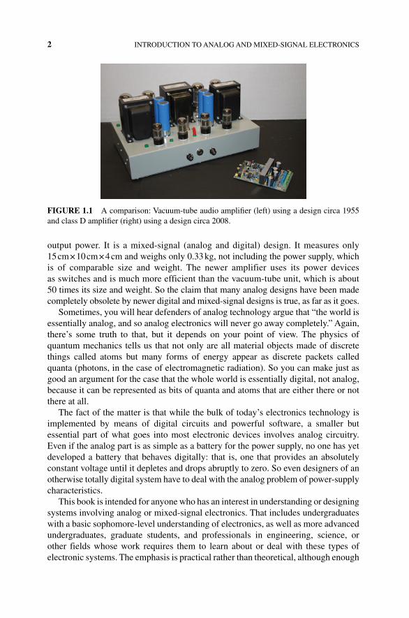