masyarakat indonesia - anupeople.anu.edu.au/budy.resosudarmo/2011to2015/amalia_reso_2013.pdf ·...

Masyarakat Indonesia Volume 39, No. 2, Desember 2013

LEMBAGA ILMU PENGETAHUAN INDONESIAYAYASAN PUSTAKA OBOR INDONESIA

JAKARTA, 2014

00-MI-39,-No 2-2013.indd 1 4/10/2014 2:15:18 PM

Masyarakat Indonesia, Volume 39, No. 2, Desember 2013 | iii

MASYARAKAT INDONESIAMAJALAH ILMU-ILMU SOSIAL INDONESIA

Volume 39 No. 2, Desember 2013

TABLE OF CONTENTS

• Acknowledgments v-vi• A foreword by IPSK Deputy Aswatini vii-viii• In Memoriam Thee Kian Wie J. Thomas Lindblad and Siwage Dharma Negara ix-xii• A foreword by the Guest Editors: Professor Anne Booth, Eminent and Prolific Scholar, Generous Friend and Colleague J. Thomas Lindblad and Thee Kian Wie xiii-xviii

1. ‘The Indonesian economy during the Soeharto era: A review’ Peter McCawley 269-2882. ‘By the numbers: Makassar’s trade, centralized statistics and local realities’ Heather Sutherland 289-3063. ‘Why was the Dutch legacy so poor? Educational development in the Netherlands Indies, 1871-1942’ Ewout Frankema 307-3264. ‘The Indonesia Economy during the Japanese Occupation’ Thee Kian Wie 327-3405. ‘A Malaysian perspective on decolonization: Lessons for Indonesia?’ J. Thomas Lindblad 341-360

00-MI-39,-No 2-2013.indd 3 4/10/2014 2:15:18 PM

6. ‘In Search of New Opportunities: The Indonesianisasi of Economic Life in Yogyakarta in the 1950s’ Bambang Purwanto 361-3787. ‘An Agricultural Development Legacy Unrealized by Five Presidents 1966-2014’ Sediono Tjondronegoro 379-3968. ‘Indonesia’s Fuel Subsidy: A Sad History of Massive Policy Failure’ Howard Dick 397-4169. ‘Ethnic Identity and Land Utilization: A Case Study in Riau, Indonesia’ Joan Hardjono 417-43610. ‘Indonesia’s Achilles Heel in the first decade of the 2000s: Employment and Labour Productivity in Manufacturing’ Chris Manning 437-45811. ‘Southeast Asian macroeconomic management: Pragmatic orthodoxy?’ Hal Hill 459-48012. ‘Indonesia’s demographic dividend or window of opportunity?’ Mayling Oey-Gardiner and Peter Gardiner 481-50413. ‘Population history in a dangerous environment: How important may natural disasters have been?’ Anthony Reid 505-52614. ‘The Consequences of Urban Air Pollution for Child Health: What does Self-Reporting Data in the Jakarta Metropolitan Area Reveal?’ Budy Resosudarmo, Mia Amalia and Jeff Bennett 527-55015. ‘The Institutionalisation of Macroeconomic Measurement in Indonesia Before The 1980s’ Pierre van der Eng 551-580

Biodata 579-586

iv | Masyarakat Indonesia, Volume 39, No. 2, Desember 2013

00-MI-39,-No 2-2013.indd 4 4/10/2014 2:15:18 PM

Masyarakat Indonesia, Volume 39, No. 2, Desember 2013 | 527

THE CONSEQUENCES OF URBAN AIR POLLUTION FOR CHILD HEALTH: WHAT DOES

SELF-REPORTING DATA IN THE JAKARTA METROPOLITAN AREA REVEAL?

Mia Amalia, Budy P. Resosudarmo and Jeff Bennett National Development Planning Agency (BAPPENAS)

Australian National University

ABSTRACT

Since the early 1990s, the air pollution level in the Jakarta Metropolitan Area has arguably been one of the highest in developing countries. This article utilizes self- reporting data on illnesses available in the 2004 National Socio-Economic Household Survey to test the hypothesis that air pollution impacts human health, particularly among children. Test results confirm that air pollution, represented by the PM10 level in a sub-district, significantly correlates with the level of human health problems, represented by the number of restricted activity days (RAD) in the previous month. Results show that the younger the person, the higher the number of RAD in the previous month; that is the impact of a given level of PM10 concentration is more hazardous for children.Keywords: Air pollution, Environmental economics, Health economics, Exposure response model

INTRODUCTION

For more than four decades Anne Booth has studied various aspects of the Indonesian economy, including issues related to land use, agriculture, labour, poverty, income inequality, regional development and fiscal policy. Fellow researchers acknowledge that her work has enriched and strengthened the scientific literature on the Indonesian economy. However, as far as the authors are aware, there is one Indonesian topic — an environmental issue — that Anne has never tackled. This article concerns the problems caused

00-MI-39,-No 2-2013.indd 527 4/10/2014 2:15:37 PM

528 | Masyarakat Indonesia, Volume 39, No. 2, Desember 2013

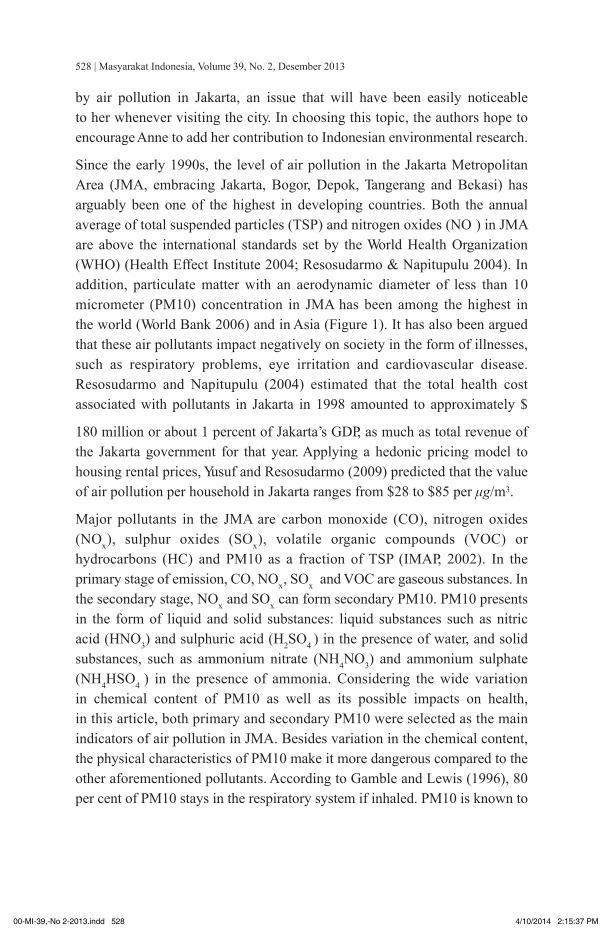
by air pollution in Jakarta, an issue that will have been easily noticeable to her whenever visiting the city. In choosing this topic, the authors hope to encourage Anne to add her contribution to Indonesian environmental research.

Since the early 1990s, the level of air pollution in the Jakarta Metropolitan Area (JMA, embracing Jakarta, Bogor, Depok, Tangerang and Bekasi) has arguably been one of the highest in developing countries. Both the annual average of total suspended particles (TSP) and nitrogen oxides (NO ) in JMA are above the international standards set by the World Health Organization (WHO) (Health Effect Institute 2004; Resosudarmo & Napitupulu 2004). In addition, particulate matter with an aerodynamic diameter of less than 10 micrometer (PM10) concentration in JMA has been among the highest in the world (World Bank 2006) and in Asia (Figure 1). It has also been argued that these air pollutants impact negatively on society in the form of illnesses, such as respiratory problems, eye irritation and cardiovascular disease. Resosudarmo and Napitupulu (2004) estimated that the total health cost associated with pollutants in Jakarta in 1998 amounted to approximately $

180 million or about 1 percent of Jakarta’s GDP, as much as total revenue of the Jakarta government for that year. Applying a hedonic pricing model to housing rental prices, Yusuf and Resosudarmo (2009) predicted that the value of air pollution per household in Jakarta ranges from $28 to $85 per μg/m3.

Major pollutants in the JMA are carbon monoxide (CO), nitrogen oxides (NOx), sulphur oxides (SOx), volatile organic compounds (VOC) or hydrocarbons (HC) and PM10 as a fraction of TSP (IMAP, 2002). In the primary stage of emission, CO, NOx, SOx and VOC are gaseous substances. In the secondary stage, NOx and SOx can form secondary PM10. PM10 presents in the form of liquid and solid substances: liquid substances such as nitric acid (HNO3) and sulphuric acid (H2SO4 ) in the presence of water, and solid substances, such as ammonium nitrate (NH4NO3) and ammonium sulphate (NH4HSO4 ) in the presence of ammonia. Considering the wide variation in chemical content of PM10 as well as its possible impacts on health, in this article, both primary and secondary PM10 were selected as the main indicators of air pollution in JMA. Besides variation in the chemical content, the physical characteristics of PM10 make it more dangerous compared to the other aforementioned pollutants. According to Gamble and Lewis (1996), 80 per cent of PM10 stays in the respiratory system if inhaled. PM10 is known to

00-MI-39,-No 2-2013.indd 528 4/10/2014 2:15:37 PM

| 529

cause respiratory diseases, especially in children with asthma (Sirikijpanichkul et al. 2006).

Figure 1Five-year (2000-2004) averages of PM10, SO2 and NO2 concentration in se-

lected Asian cities

Source: Health Effect Institute 2010.

This article focuses on the quantification of PM10 impacts on child health, using the number of restricted activity days (RAD) as the unit of analysis. Children are the focus of this article since, particularly in developing countries, they are the group most vulnerable to health related air quality problems due to their relatively high exposure to the low quality of air and their under- developed immune system (World Research Institute 1999; Haryanto, 2007). The types of illnesses considered are lower and upper respiratory illnesses. In this research, the causal relationship between PM10 and respiratory illnesses was estimated using dose-response functions or exposure response models (ERM) (Resosudarmo & Napitupulu 2004).

Hospital and health center data on health impacts caused by air pollutants in most developing countries are not an accurate representation of the actual number of people affected, since many prefer to visit private doctors or to buy pharmacy medicines (Frankenberg et al. 2005). Other reasons to avoid using such data are that collecting patient data from all hospitals and health centres in big cities in developing countries is time consuming and would not comply with the scientific research ethical directive regarding

Mia Amalia, Budy P. Resosudarmo And Jeff Bennett | The Consequences Of Urban ....

00-MI-39,-No 2-2013.indd 529 4/10/2014 2:15:38 PM


data released from hospital and other public facilities to the researcher as the third party. As a result, this paper utilizes the self-reporting data on illnesses available in the 2004 National Socio-Economic Household Survey (Survei Sosial Ekonomi Nasional, SUSENAS) to develop an ERM estimating the impact of air pollution on human health, particularly among children, in the JMA. The indicator used to represent air pollution is PM10, while its impact on human health is represented by the number of restricted activity days (RAD) in the past month caused by lower and upper respiratory tract infections. SUSENAS is a large-scale, nationally representative, repeated cross-section survey conducted since the 1960s. In this article, the current literature on the public health impacts and risk assessment of air pollution is reviewed in Sections 2 and 3, respectively. Section 4 provides modelling results and Section 5 concludes the paper.

AIR POLLUTION IMPACTS ON HUMAN HEALTH

The literature on the impacts of air pollution on human health, in general, believes that the most damaging pollutant to human health is PM10 (Gamble & Lewis 1996). PM in the form of TSP, PM10, PM2.5, NOx and SOx is related to upper respiratory tract symptoms, such as cough, bronchitis and chest infection especially in young children. These pollutants are also closely linked to lower respiratory tract system conditions, such as asthma. With higher PM concentrations in urban areas, asthma becomes more common, especially in children (Koren & Utell 1997).

Hospital admissions for asthma attack show a positive relationship with PM from two days to a week’s lag time. Asthma causes the loss of approximately three million working days and 90 million RAD annually in big cities in the USA (Pope et al. 1995). Asthma attacks are also considered to cause death, although a study by Koren and Utell (1997), using the total number of deaths and the average PM10 concentration per year, could not establish the relationship between these factors. For instance, in the United States, asthma deaths increased from 1979 to 1989, while PM10 and SOx average concentrations decreased (Koren & Utell 1997).

Deposition of PM in lungs can cause lung inflammation and cytokine release affecting heart activity and can further cause cardiac arrest. Due to its ability to deposit in the lungs, PM10 is also a threat to the

00-MI-39,-No 2-2013.indd 530 4/10/2014 2:15:38 PM

| 531

elderly and children. It has been associated with hospital admission and emergency room visits for chronic obstructive pulmonary disease (COPD), pneumonia and cardiovascular disease, such as ischemic heart disease (IHD) (Brumback et al.,2000; Samet et al. 2000; Schwartz 1995). A study conducted in the United States concluded that the effect of TSP — including PM10 and PM2.5 — on adult mortality is large and positive (Chay et al. 2003). Researchers agree that the smaller the particles, the more dangerous they are (Dockery et al. 1995; Marrack 1995; Pope et al. 1996) since the chance of them being deeply inhaled is greater. McCubbin and Delucchi (1996) argue that PM contributes the most to health costs. Therefore, they conclude that stronger regulation of particulates will reduce mortality and morbidity.

On modelling the relationship between air pollutants and human health or ERM, the literature concludes that pollutant concentration can be used in single pollutant models. However, an aggregation of several single air pollutant models can overestimate the overall health outcomes and cause double counting in economic analysis (Kneese 1984; Kunzli et al. 2000). All the same, the use of a single indicator alone may underestimate the value of health impacts, it may disregard effects of other pollutants which are independent of the selected pollutant (Kunzli et al. 2000). To estimate the correct value of ambient air improvement, researchers have developed a different pollutant combination to value the total impacts of air pollutants on human health. Some use a surrogate pollutant to estimate some or all of the effects of all the other pollutants (BTRE 2005). For instance, Kunzli et al. (2000) use PM10 only because they argue that PM10 is a reliable indicator of several sources of outdoor air pollution. Other researchers agree with this approach, for several reasons:

1. PM10 is used as the surrogate pollutant for SO2, CO and NO2 since PM10 is correlated significantly with SO2, CO and NO2 and not with O3 and because acid pollutants such as SO2 and NO2 contribute to the formation of PM10.

2. PM10 is used as a surrogate because PM10 is a respirable air pollutant and an important contributing factor to respiratory disease with a strong relationship to mortality.

3. PM10 is a complex pollutant since it is a ‘heterogeneous mix of solid or liquid compounds’ such as organic aerosols, primary and secondary


00-MI-39,-No 2-2013.indd 531 4/10/2014 2:15:38 PM


pollutants, and metal. This property implies that PM10 is a surrogate measure for one of its components or for other pollutants.

The literature agrees that PM10 or PM2.5 is the best estimator for calculating the health effects of air pollution (Peters & Dockery 2006). The first reason for this is its close relationship with mortality and morbidity. The second reason is that secondary PM10 also consists of transition compounds of SOx and NOx in the form of ammonium sulphate and ammonium nitrate. This paper, hence, will use PM10 as the measure of air pollution to estimate the human health impacts of air pollution in the JMA.

METHOD: RISK ASSESSMENT FOR PUBLIC HEALTH

ERM estimation is one of the processes used in Risk Assessment for Public Health. The complete process of this risk assessment includes first, determining the average annual concentration of each pollutant over a period of time; second, calculating the health impact and estimating the relationship between the pollutants and the health impact. This is carried out through the following sub-steps:

(1) identification of health hazards by calculating the number of deaths, hospital admissions, or other health outcomes during a certain period of time (Samet et al. 1994);

(2) estimation of the ERM;

(3) estimation of the population’s profile of exposure to the health hazard.

The last step of this risk assessment is aggregating health risk in the form of a monetary unit (Samet et al. 1994).

As this article intends to develop an ERM, it only applies the second step with its sub-steps, using cross sectional data analysis of the aforementioned risk assessment process. Cross sectional analysis uses pollutant level data from different areas and relates them to the morbidity levels within the corresponding area. The general model of an ERM is a multivariate model as follows (Frankenberg et al. 2005);

00-MI-39,-No 2-2013.indd 532 4/10/2014 2:15:38 PM

| 533

where: hi is whether or not an individual was impacted by the air quality. Appropriate models for Equation 1 are probit or multinomial models. pi is an index measuring the level of air pollution exposure. Xi is a matrix of various individual and village socio-economic characteristics (Frankenberg et al. 2005). Zi is a matrix containing levels or proxies of indoor air pollution or other pollutants. Zi is meant to resolve the issue of omitting variable bias that commonly occurs in ERM models. Meanwhile ei is white random errors. The main hypothesis is that α1 is equal to zero.

In addition, a population profile analysis was added to determine the most affected and sensitive groups in a population. Sensitive groups such as infants and elderly people might react differently from other groups to the same exposure. To gain a complete estimation an ERM must consider the total dose received by certain groups in the entire population. The population profile is based on: individual physical and health conditions; individual habits and activities; socio-demographic and socio-economic characteristics as well as housing including sources of indoor air pollution and community or neighbourhood conditions.

DATA CONSTRUCTION

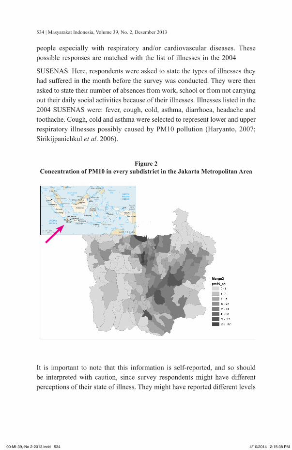
PM10 is identified as the surrogate pollutant to represent all main pollutants in JMA. Average annual concentration of PM10 is estimated using a PM10 Dispersion Model (PMDM). This model is developed by combining two available dispersion models: the Simplified Mobile Emission Model (SIMEM) and the Simple Interactive Model for Better Air Quality (SIM-AIR). Figure 2 shows the ambient level of PM10 in 2004 resulting from the PMDM utilized in this article.

All possible health hazards caused by PM10 are identified and listed. According to Sirikijpanichkul et al. (2006), human responses to PM10 pollution are: mortality, morbidity, chronic and acute bronchitis, hospital admissions, lower and upper respiratory illnesses, chest pain, respiratory symptoms, minor and major RAD, and asthma affecting children and elderly


00-MI-39,-No 2-2013.indd 533 4/10/2014 2:15:38 PM


people especially with respiratory and/or cardiovascular diseases. These possible responses are matched with the list of illnesses in the 2004

SUSENAS. Here, respondents were asked to state the types of illnesses they had suffered in the month before the survey was conducted. They were then asked to state their number of absences from work, school or from not carrying out their daily social activities because of their illnesses. Illnesses listed in the 2004 SUSENAS were: fever, cough, cold, asthma, diarrhoea, headache and toothache. Cough, cold and asthma were selected to represent lower and upper respiratory illnesses possibly caused by PM10 pollution (Haryanto, 2007; Sirikijpanichkul et al. 2006).

Figure 2Concentration of PM10 in every subdistrict in the Jakarta Metropolitan Area

It is important to note that this information is self-reported, and so should be interpreted with caution, since survey respondents might have different perceptions of their state of illness. They might have reported different levels

00-MI-39,-No 2-2013.indd 534 4/10/2014 2:15:38 PM

| 535

of illness using a uniform unit: number of days of absence or restricted activity days (RAD).

The 2004 SUSENAS also contains data on the population profile. Proxies for the population profile are grouped into: individual physical and health condition; individual activities and habits; socio-demographic and socioeconomic characteristics; indoor pollution; as well as house and community conditions. Proxies for each group are as follows:

1 individual physical and health status: parents’ and siblings’ health status a month before the survey was conducted;

2 individual activities and habits: smoking habit, number of cigarettes smoked per day, number of years of routine smoking, members of the family who smoke indoors, family smoking habit;

3 socio-demographic and socioeconomic characteristics: expenditure, expenditure per capita, head of household’s education, occupation and income and average working hours per week; and

4 house condition, indoor pollution and community conditions which include:

a. proxies for house condition: ceiling, age, wall, floor, density, function, land/house area ratio;

b. proxies for indoor pollutants: sprays, disinfectants, bleach, batteries, paint, insecticides; and

c. proxies for community conditions: location, disaster area, access to street, street width, street cover materials, community average expenditure, average distance to community facilities such as primary schools, community health centres and sub-district offices.

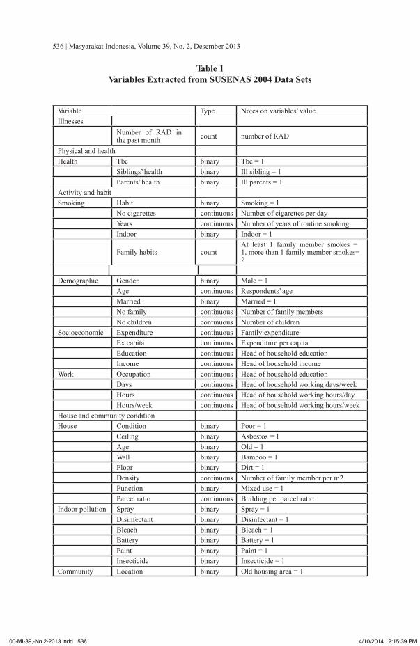
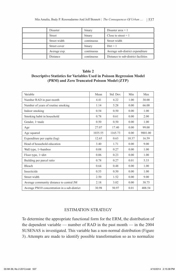
The list of final variables extracted from the 2004 SUSENAS dataset are presented in Table 1 and the list of variables used in the model with their descriptive statistics are presented in Table 2.


00-MI-39,-No 2-2013.indd 535 4/10/2014 2:15:38 PM


Table 1Variables Extracted from SUSENAS 2004 Data Sets

Variable Type Notes on variables’ valueIllnesses

Number of RAD in the past month count number of RAD

Physical and healthHealth Tbc binary Tbc = 1

Siblings’ health binary Ill sibling = 1Parents’ health binary Ill parents = 1

Activity and habitSmoking Habit binary Smoking = 1

No cigarettes continuous Number of cigarettes per dayYears continuous Number of years of routine smokingIndoor binary Indoor = 1

Family habits countAt least 1 family member smokes = 1, more than 1 family member smokes= 2

Demographic Gender binary Male = 1Age continuous Respondents’ ageMarried binary Married = 1No family continuous Number of family membersNo children continuous Number of children

Socioeconomic Expenditure continuous Family expenditureEx capita continuous Expenditure per capitaEducation continuous Head of household educationIncome continuous Head of household income

Work Occupation continuous Head of household educationDays continuous Head of household working days/weekHours continuous Head of household working hours/dayHours/week continuous Head of household working hours/week

House and community conditionHouse Condition binary Poor = 1

Ceiling binary Asbestos = 1Age binary Old = 1Wall binary Bamboo = 1Floor binary Dirt = 1Density continuous Number of family member per m2Function binary Mixed use = 1Parcel ratio continuous Building per parcel ratio

Indoor pollution Spray binary Spray = 1Disinfectant binary Disinfectant = 1Bleach binary Bleach = 1Battery binary Battery = 1Paint binary Paint = 1Insecticide binary Insecticide = 1

Community Location binary Old housing area = 1

00-MI-39,-No 2-2013.indd 536 4/10/2014 2:15:39 PM

| 537

Disaster binary Disaster area = 1

Street binary Close to street = 1

Street width continuous Street width

Street cover binary Dirt = 1

Average exp. continuous Average sub-district expenditure

Distance continuous Distance to sub-district facilities

Table 2Descriptive Statistics for Variables Used in Poisson Regression Model

(PRM) and Zero Truncated Poisson Model (ZTP)

Variable Mean Std. Dev. Min Max

Number RAD in past month 4.41 4.22 1.00 30.00

Number of years of routine smoking 1.14 5.28 0.00 66.00

Indoor smoking 0.54 0.50 0.00 1.00

Smoking habit in household 0.78 0.61 0.00 2.00

Gender, 1=male 0.50 0.50 0.00 1.00

Age 27.07 17.40 0.00 99.00

Age squared 1035.55 1165.73 0.00 9801.00

Expenditure per capita (log) 12.65 0.63 10.37 16.59

Head of household education 3.40 1.71 0.00 9.00

Wall type, 1=bamboo 0.08 0.27 0.00 1.00

Floor type, 1=dirt 0.06 0.23 0.00 1.00

Building per parcel ratio 0.78 0.27 0.01 5.33

Bleach 0.64 0.48 0.00 1.00

Insecticide 0.55 0.50 0.00 1.00

Street width 2.50 1.52 0.00 9.00

Average community distance to central JM 2.18 3.02 0.00 38.75

Average PM10 concentration in a sub-district 30.98 50.97 0.01 408.54

ESTIMATION STRATEGY

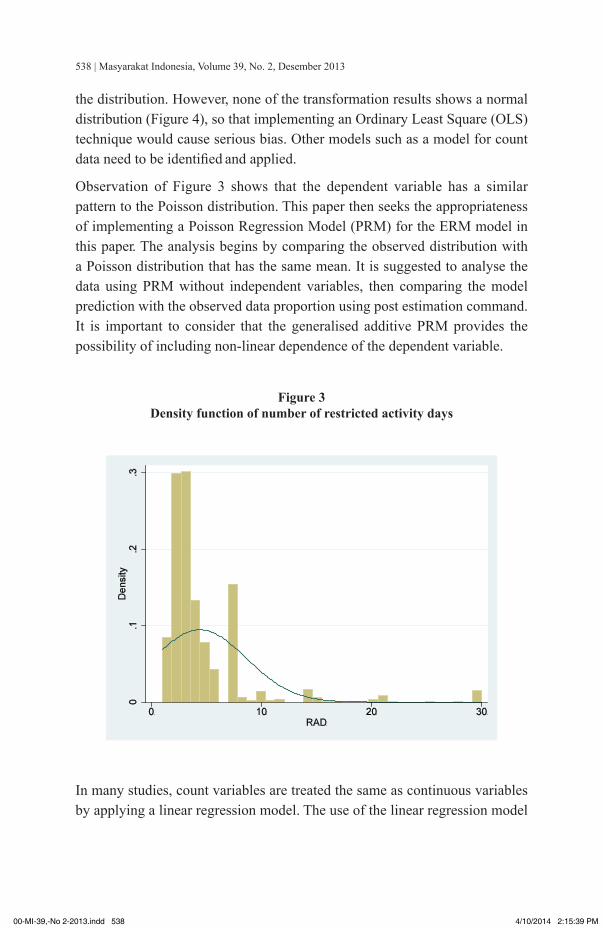
To determine the appropriate functional form for the ERM, the distribution of the dependent variable — number of RAD in the past month — in the 2004 SUSENAS is investigated. This variable has a non-normal distribution (Figure 3). Attempts are made to identify possible transformation so as to normalize


00-MI-39,-No 2-2013.indd 537 4/10/2014 2:15:39 PM


the distribution. However, none of the transformation results shows a normal distribution (Figure 4), so that implementing an Ordinary Least Square (OLS) technique would cause serious bias. Other models such as a model for count data need to be identified and applied.

Observation of Figure 3 shows that the dependent variable has a similar pattern to the Poisson distribution. This paper then seeks the appropriateness of implementing a Poisson Regression Model (PRM) for the ERM model in this paper. The analysis begins by comparing the observed distribution with a Poisson distribution that has the same mean. It is suggested to analyse the data using PRM without independent variables, then comparing the model prediction with the observed data proportion using post estimation command. It is important to consider that the generalised additive PRM provides the possibility of including non-linear dependence of the dependent variable.

Figure 3Density function of number of restricted activity days

In many studies, count variables are treated the same as continuous variables by applying a linear regression model. The use of the linear regression model

00-MI-39,-No 2-2013.indd 538 4/10/2014 2:15:39 PM

| 539

can cause a biased, inefficient and inconsistent estimate. In a case where the amount of zero observation exceeds the allowable number, a zero inflated model for PRM is applied. On the other hand, when there are no zeros, a truncated version needs to be applied.

Figure 4Transformations of the dependent variable: Number of restricted

activity days

The results from data analysis using PRM without independent variables (solid line in Figure 5) indicate that the observed proportion shows that respondents tended to choose ‘convenient numbers’ for RAD such as one week, two weeks, three weeks and one month represented by seven, fourteen, twenty one and thirty days, respectively. Three days has the highest probability: a possible explanation for this condition is that doctors usually recommend staying home for a maximum of three days in a letter addressed to the employer or school administrator.


00-MI-39,-No 2-2013.indd 539 4/10/2014 2:15:39 PM


Figure 5Comparison between real data and Poisson prediction

The prediction results using PRM (dash line in Figure 5), show a smoother graph reducing extreme probability at three, seven, fourteen, twenty one and thirty days of RAD. It can be seen that PRM is relatively appropriate to be utilized with the data set available for this article.

The minimum number of RAD is one day and the maximum is thirty days, therefore an estimation using Zero Truncated Poisson Regression Model (ZTP) is also utilized.

In estimating the ERM, this article will, first, utilize the overall sample in the 2004 SUSENAS to observe the health impact of air pollutants on the overall population of JMA. After that a focus on the impact of air pollutants on child health is conducted. Children are defined as family members aged of fourteen or under. A comparison with the impact on non-head of household adults and the elderly group is conducted. Adults are those aged between fourteen and sixty. Elderly is defined as sixty and older. The main reason for removing the household head from the adult group is that they typically spend most of their day at a work place and/or travelling outside their sub-districts; meaning they

00-MI-39,-No 2-2013.indd 540 4/10/2014 2:15:40 PM

| 541

are most likely exposed to a different level of air pollutant to their children. On the other hand, non-head of household adults and the elderly are most likely exposed to the same air pollutants as their children.

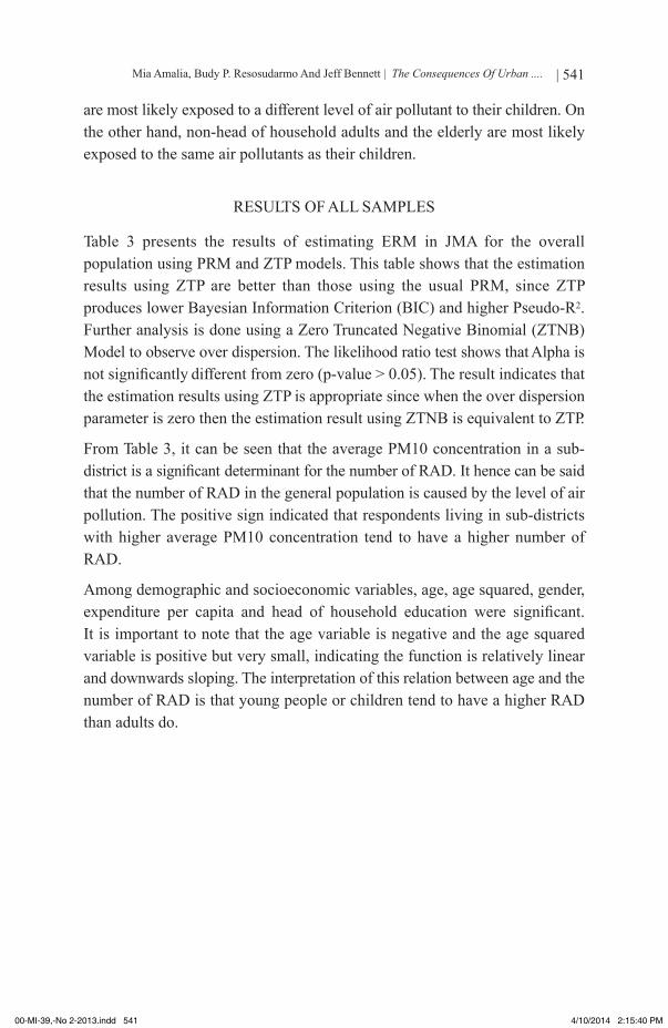
RESULTS OF ALL SAMPLES

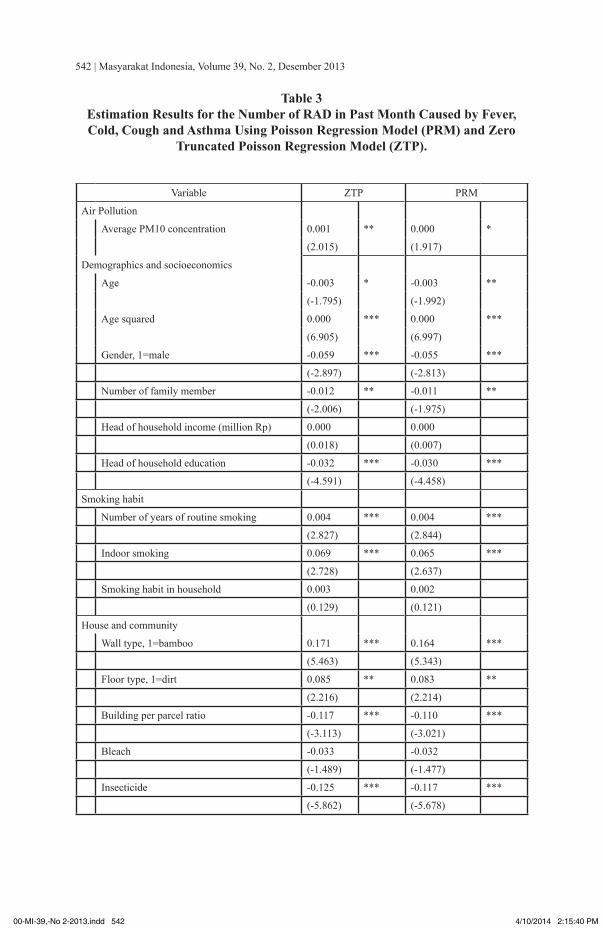
Table 3 presents the results of estimating ERM in JMA for the overall population using PRM and ZTP models. This table shows that the estimation results using ZTP are better than those using the usual PRM, since ZTP produces lower Bayesian Information Criterion (BIC) and higher Pseudo-R2. Further analysis is done using a Zero Truncated Negative Binomial (ZTNB) Model to observe over dispersion. The likelihood ratio test shows that Alpha is not significantly different from zero (p-value > 0.05). The result indicates that the estimation results using ZTP is appropriate since when the over dispersion parameter is zero then the estimation result using ZTNB is equivalent to ZTP.

From Table 3, it can be seen that the average PM10 concentration in a sub- district is a significant determinant for the number of RAD. It hence can be said that the number of RAD in the general population is caused by the level of air pollution. The positive sign indicated that respondents living in sub-districts with higher average PM10 concentration tend to have a higher number of RAD.

Among demographic and socioeconomic variables, age, age squared, gender, expenditure per capita and head of household education were significant. It is important to note that the age variable is negative and the age squared variable is positive but very small, indicating the function is relatively linear and downwards sloping. The interpretation of this relation between age and the number of RAD is that young people or children tend to have a higher RAD than adults do.


00-MI-39,-No 2-2013.indd 541 4/10/2014 2:15:40 PM


Table 3Estimation Results for the Number of RAD in Past Month Caused by Fever, Cold, Cough and Asthma Using Poisson Regression Model (PRM) and Zero

Truncated Poisson Regression Model (ZTP).

Variable ZTP PRM

Air Pollution

Average PM10 concentration 0.001 ** 0.000 *

(2.015) (1.917)

Demographics and socioeconomics

Age -0.003 * -0.003 **

(-1.795) (-1.992)

Age squared 0.000 *** 0.000 ***

(6.905) (6.997)

Gender, 1=male -0.059 *** -0.055 ***

(-2.897) (-2.813)

Number of family member -0.012 ** -0.011 **

(-2.006) (-1.975)

Head of household income (million Rp) 0.000 0.000

(0.018) (0.007)

Head of household education -0.032 *** -0.030 ***

(-4.591) (-4.458)

Smoking habit

Number of years of routine smoking 0.004 *** 0.004 ***

(2.827) (2.844)

Indoor smoking 0.069 *** 0.065 ***

(2.728) (2.637)

Smoking habit in household 0.003 0.002

(0.129) (0.121)

House and community

Wall type, 1=bamboo 0.171 *** 0.164 ***

(5.463) (5.343)

Floor type, 1=dirt 0.085 ** 0.083 **

(2.216) (2.214)

Building per parcel ratio -0.117 *** -0.110 ***

(-3.113) (-3.021)

Bleach -0.033 -0.032

(-1.489) (-1.477)

Insecticide -0.125 *** -0.117 ***

(-5.862) (-5.678)

00-MI-39,-No 2-2013.indd 542 4/10/2014 2:15:40 PM

| 543

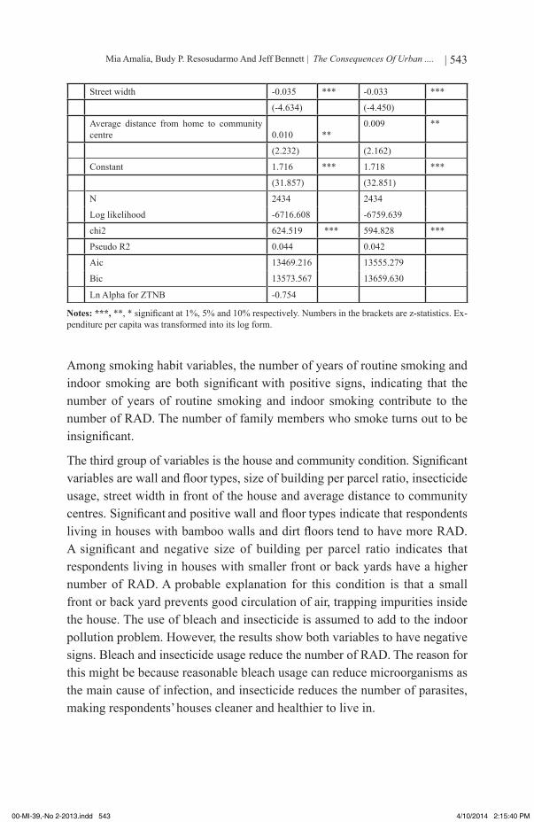
Street width -0.035 *** -0.033 ***

(-4.634) (-4.450)

Average distance from home to community centre 0.010 **

0.009 **

(2.232) (2.162)

Constant 1.716 *** 1.718 ***

(31.857) (32.851)

N 2434 2434

Log likelihood -6716.608 -6759.639

chi2 624.519 *** 594.828 ***

Pseudo R2 0.044 0.042

Aic 13469.216 13555.279

Bic 13573.567 13659.630

Ln Alpha for ZTNB -0.754

Notes: ***, **, * significant at 1%, 5% and 10% respectively. Numbers in the brackets are z-statistics. Ex-penditure per capita was transformed into its log form.

Among smoking habit variables, the number of years of routine smoking and indoor smoking are both significant with positive signs, indicating that the number of years of routine smoking and indoor smoking contribute to the number of RAD. The number of family members who smoke turns out to be insignificant.

The third group of variables is the house and community condition. Significant variables are wall and floor types, size of building per parcel ratio, insecticide usage, street width in front of the house and average distance to community centres. Significant and positive wall and floor types indicate that respondents living in houses with bamboo walls and dirt floors tend to have more RAD. A significant and negative size of building per parcel ratio indicates that respondents living in houses with smaller front or back yards have a higher number of RAD. A probable explanation for this condition is that a small front or back yard prevents good circulation of air, trapping impurities inside the house. The use of bleach and insecticide is assumed to add to the indoor pollution problem. However, the results show both variables to have negative signs. Bleach and insecticide usage reduce the number of RAD. The reason for this might be because reasonable bleach usage can reduce microorganisms as the main cause of infection, and insecticide reduces the number of parasites, making respondents’ houses cleaner and healthier to live in.


00-MI-39,-No 2-2013.indd 543 4/10/2014 2:15:40 PM


Respondents living in wider streets tend to have a lower number of RAD since wider streets usually have better street cover than narrower ones and are complemented with good sewers and drainage systems, making the environment cleaner. The location of houses relative to community centres (average distance to community centres) is also significant and positive, indicating that respondents living further from community centres have a higher number of RAD. This condition indicates that the longer it takes for the respondents to reach their daily destination, the higher the number of RAD.

RESULTS FOR GROUPS

Modelling results for the number of RAD among children, adults (non-head of household) and the elderly are set out in Table 4. Observing the relationships between PM10 concentration in a sub-district and the number of RAD in the previous month among the three age groups, it can be seen that they all have a positive relationship with almost the same coefficient size. The difference is that this relationship is highly significant (with a 1 per cent significance level) among children, weakly significant among adults (with only a 10 per cent significance level), and not significant among the elderly; i.e. the impact of PM10 concentration in a sub-district on children’s health in that sub-district is much more consistent compared to that for other age groups.

For children, other significant variables are age, gender, head of household income, head of household education, and average distance from home to community centres. Again, among children, with the same level of exposure to pollution, the younger the child, the higher the number of previous month RAD.

For adult family members, other significant variables are individual smoking habits, head of household income, head of household education, wall type, street width in front of the house, and average distance from home to community centres. For elderly family members, other significant variables are individual smoking habits, gender, age, head of household education, wall type, and average distance to the community centre and types of work. For this group of respondents, older males who smoke and who come from a family where the head of the household has lower education tended to have more RAD compared to other members of the group.

00-MI-39,-No 2-2013.indd 544 4/10/2014 2:15:40 PM

| 545

Table 4Estimation Results for Number of RAD in Past Month Caused by Fe- ver, Cold,

Cough and Asthma Using Zero Truncated Poisson Regression Model (ZTP).

Variable Adult Elder ChildrenAir Pollution

Average PM10 concentration 0.001 * 0.001 0.001 ***(1.672) (0.478) (2.835)

Demographics and socioeconomicsAge 0.009 0.010 ** -0.013 ***

(4.966) (2.021) (-3.219)Gender, 1=male -0.041 0.230 *** -0.055 *

(-0.762) (3.029) (-1.728)Head of household income 0.219 *** 0.069 -0.098 *

(3.393) (0.366) (-1.684)Head of household education -0.052 *** -0.069 ** -0.076 ***

(-4.032) (-2.774) (-6.776)Health condition and habit

Individual smoking habit 0.087 * 0.306 ***(2.129) (4.106)

House and communityWall type, 1=bamboo 0.276 *** 0.402 ***

(5.050) (4.340)Street width -0.039 ***

(-2.805)Average distance from home to community centre 0.044 *** 0.027 ** 0.017 **

(5.130) (2.116) (2.586)Occupation

Worker -0.174 -0.231 **(-3.749) (-2.340)

Student 0.018(0.221)

Constant 1.297 *** 0.978 ** 1.655 ***(13.900) (2.504) (32.742)

N 674 118 1076Log likelihood -1885.881 -475.915chi2 180.706 87.126 76.183Pseudo R2 0.046 0.084 0.015aic 3797.761 977.831 5162.287bic 3856.433 1013.850 5197.154

Notes: ***, **, * significant at 1%, 5% and 10% respectively. Numbers in the brackets are z-statistics. Expenditure per capita was transformed into its log form.


00-MI-39,-No 2-2013.indd 545 4/10/2014 2:15:40 PM


A rather puzzling result is the impact of household income on the number of RAD. Among children, a higher family income means a lower number of RAD; that is something that is expected. Among adult family members, however, a higher family income means a higher number of RAD. And, among the elderly, family income is not a significant determinant of the number of RAD. Further study in this subject depends on good explanations for this result.

CONCLUSION

Impacts of PM10 pollution in JMA on health are investigated in this article. The main contribution of this paper is that it uses individual self-reporting data on health problems in the population of interest. There are problems associated with self-reporting information. Survey respondents might have different perceptions of their state of illness. They might report different levels of illness using a uniform unit. Nevertheless, the article proposes that, for developing regions such as Jakarta, information derived from self-reporting is more useful in dealing with health problems than estimations derived from using ERM programs designed for developed countries.

The ERM in this paper is estimated using a PRM and ZTP since the distribution of the dependent variable, that is number of RAD during last month, was similar to the Poisson distribution. The results from the analyses show that once a person falls ill, PM10 concentration becomes one of the causal variables in increasing or reducing the number of RAD. The relationship between PM10 in a sub-district and the number of previous month RAD, in general, is positive and significant. The results also show that the younger the person, the higher the number of previous month RAD; that is the impact of a given level of PM10 concentration is more fatal for younger persons.

To better identify the vulnerable groups, the data set is split into three groups: adult family members, children and elderly family members. The results show that children are the group most vulnerable to PM10 pollution. PM10 concentration is a highly significant causal variable in children falling ill as a result of fever, cold, cough and asthma.

00-MI-39,-No 2-2013.indd 546 4/10/2014 2:15:40 PM

| 547

BIBLIOGRAPHY

Books

Botkin, D.& Keller, E. 2005. Environmental Science. Hoboken, NJ: Wiley.Dockery, D.W., Schwartz, J.& Pope III, C. 1995. Comments from Original

Investigators, Particulate Air Pollution and Daily Mortality: Replication and Validation of Selected Studies. Cambridge, MA: Health Effects Institute.

Kneese, A. 1984. Measuring the Benefits of Clean Air and Water. Washington, DC, Resource for the Future.

Articles

Brumback, B., Ryan, L., Schwartz, J., Neas, L., Stark, P. & Burge, H. 2000. “Transitional Regression Models with Application to Environmental Time Series,”. Journal of American Statistical Association. Vol. 95, no. 449: 16-27.

Chay, K., Dobkin, C. & Greenstone, M. 2003.“The Clean Air Act of 1970 and Adult Mortality”. Journal of Risk and Uncertainty. Vol. 23, no. 3: 279-300.

Frankenberg, E., McKee, D. & Thomas, D. 2005.“Health Consequences of Forest Fires in Indonesia”. Demography. Vol. 42, no.1: 109-129.

Gamble, J.F.& Lewis, R.J. 1996. “Health and Respirable Particulate (PM10) Air Pollution: a Causal or Statistical Association?” Environmental Health Perspectives. Vol.104, no. 8: 838-850.

Haryanto, B. 2007. “Blood-lead Monitoring Exposure to Unleaded-gasoline Among School Children in Jakarta – Indonesia 2005”. Jurnal Kesehatan Masyarakat. No. 5.

Koren, H.S. & Utell, M.J. 1997.“Asthma and the Environment”. Environmental Health Perspectives. Vol.105, no. 5: 534-537.

Kunzli, N., Kaiser, R., Medina, S., Studnicka, M., Chanel, O., Filliger, P., Herry, M., Horak Jr, F., Puybonnieux-Texier, Quenel, P., Schneider, J., Seethaler, R., Vergnaud, J.-C.& Sommer, H. 2000. “Public-health Impact of Outdoor and Traffic-related Air Pollution: a European Assessment’, The Lancet. Vol. 356, no. 9232: 795-801.

McCubbin, D.R.& Delucchi, M.A. 1996. “The Health Costs of Motor-vehicle-related Air Pollution”. Journal of Transport Economics and Policy. Vol. 33, no. 3: 253-286.

Peters, A.& Dockery, D.W. 2006. “Air Pollution and Health Effects: Evidence from Epidemiologic Studies”. In W. Foster & D. Costa (editors), Air Pollutants and the Respiratory Tract. Boca Raton, LA; Taylor and Francis.


00-MI-39,-No 2-2013.indd 547 4/10/2014 2:15:40 PM


Pope III, C., Bates, D.V.& Raizenne, M.E. 1995. “Health Effects of Particulate Air Pollution: Time for Reassessment?”. Environmental Health Perspectives. Vol. 103, no. 5: 472-480.

Pope III, C., Thun, M., Namboodiri, M., Dockery, D.W., Evans, C.D., Speizer, F.E.& Heath, C. 1996. “Particulate Air Pollution as a Predictor of Mortality in the Perspective Study of US Adults”. American Journal of Respiratory and Critical Care Medicine. Vol. 151: 669-674.

Resosudarmo, B.P. & Napitupulu, L. 2004. “Health and Economic Impact of Air Pollution in Jakarta”. Economic Record. Vol. 80 [Special issue]: S65-S75.

Schwartz, J. 1995.“Air Pollution and Hospital Admissions to the Elderly in Birmingham, Alabama”. American Journal of Epidemiology. Vol.139: 589-598.

Yusuf, A.A. and Resosudarmo, B.P. 2009, “Does clean air matter in developing countries’ megacities? A hedonic price analysis of the Jakarta housing market, Indonesia.’, Ecological Economics, Vol. 68, pp. 1398-1407.

Reports and Presentations

Bureau of Transportation and Regional Economics (BTRE). 2005. Working paper 63: Health Impacts of Transport Emissions in Australia: Economic Costs. Canberra: Department of transport and regional services.

Health Effect Institute. 2004. Health Effects of Outdoor Air Pollution in Developing Countries of Asia: a Literature Review. [Special Report 15]. Boston: Health Effect Institute.

--------. 2010. Outdoor Air Pollution and Health in the Developing Countries of Asia: a Comprehensive Review. [Special Report 18]. Boston: Health Effect Institute.

Indonesian Multi-sectoral Action Plan (IMAP) Group on Vehicle Emissions Reduction (IMAP). 2002. Action Plan: Integrated Vehicle Emission Reduction Strategy for Greater Jakarta. Jakarta: Asian Development Bank.

Marrack, D. 1995.“All PM10 are not Biological Equal”. International Conference on Particulate Matter, Health and Regulatory Issues, Pittsburgh.

Samet, J., Zeger, S., Dominici, F., Curriero, F., Coursac, I., Dockery, D.W., Schwartz, J.& Zanobetti, A. 2000. National Morbidity, Mortality, and Air Pollution Study II: Morbidity, Mortality and Air Pollution in the United States. North Andover, MA: Health Effect Institute.

Sirikijpanichkul, A., Iyengar, M.& Ferreira, L. 2006.Valuing Air Quality Impacts of Transportation: a Review of Literature. Brisbane: School of Urban Development, Queensland University of Technology.

Surbakti, P. 1995. Indonesia’s National Socio-economic Survey: a Continual Data Source for Analysis on Welfare Development. Jakarta: Central Bureau of Statistics.

00-MI-39,-No 2-2013.indd 548 4/10/2014 2:15:41 PM

| 549

Websites

World Bank. 2006. World Development Indicators [viewed 3 November 2008]. http://devdata.worldbank.org

World Resource Institute. 1999. “Urban Air Pollution Risks to Children: A Global Environmental Health Indicator”. [viewed 2 April 2012].http://www.wri.org


00-MI-39,-No 2-2013.indd 549 4/10/2014 2:15:41 PM

masyarakat indonesia - anupeople.anu.edu.au/budy.resosudarmo/2011to2015/amalia_reso_2013.pdf ·...

Documents