illustrative subsidy variations to attract investors ... · share of bananas eaten in kalimantan...
TRANSCRIPT

387Illustrative Subsidy Variations to Attract Investors
A b s t r a c t
ILLUSTRATIVE SUBSIDY VARIATIONSTO ATTRACT INVESTORS
(using the EMERALD Indonesian multi-regional CGE model)
Daniel PambudiAndi Alfian Parewangi1
Paper ini membahas dampak ekonomi dari subsidi terhadap industri yang dapat menarik minat
investor pada daerah tertentu. Dengan mempergunakan EMERALD (Equilibrium Model with Economic
Regional Analysis Dimensions) yang merupakan model CGE multi region untuk Indonesia, paper ini
menganalisa beberapa simulasi alternatif pembiayaan subsidi industri Tekstil di Jawa Tengah.
Hasil yang diperoleh menunjukkan bahwa subsidi atas industri Tekstil dengan sumber pendanaan
bukan pajak akan meningkatkan daya saing industri Tekstil diatas biaya sektor tradable secara
keseluruhan. Secara riil, subsidi ini akan meningkatkan PDRB Jawa Tengah sebesar 0.21%. Jika
subsidi tersebut dibiayai dari pengenaan pajak atas rumah tangga, akan meningkatkan PDRB Jawa
Tengah sebesar 0.11%.
Keyword: Regional, Computable General Equilibrium, investment, subsidy
JEL: C68, D92, E62, O18
1 Pambudi is PhD student at the Centre of Policy Studies (CoPS), Monash University, supervised by Dr. Mark Horridge.Pambudi’s interest is in the application of multi-sectoral and multi-regional economic model for policy analysis. AndiAlfian Parewangi was visiting scholar at CoPS, Monash University under supervision of Dr. Glyn Wittwer and also lecturerat Department of Economic, University of Indonesia.

388 Buletin Ekonomi Moneter dan Perbankan, Desember 2004
1. BACKGROUND1.1. Introduction
The aim of this research is to construct a bottoms-up CGE model for Indonesia that
can be used for studying and analysing regional policies comprehensively. This model makes
us possible to simulate regional based polices scenario to obtain the regional and national
results.
This model adopts the TERM model structure for comparative static analyses. We
use the new model to study the policy implications of competitive bidding between regions
to attract investment. Tax concessions, for instance, are sometimes viewed as an attractive
instrument to boost regional and national welfare. However, national approaches differ. For
example, Australian states subsidize some investors and the Federal Government taxes
them. Vietnam taxes them. The model may suggest which approach is better. Also, the
long-run effects of taxing (or subsidizing) investments may differ from the short-run effects.
Again, national interest may conflict with those of individual regions. The model will be used
to examine some of these issues.
To construct this big multiregional model, we require data on regional supplies and
demands. Moreover, the necessary inter-regional flows data showing, for example, what
share of bananas eaten in Kalimantan come from Java are rarely available. To overcome
these problems, innovations will be needed. In preparing and making data which used for
this model, we adopt a data making process from Horridge, such as using the gravity approach
to produce inter-regional data.
Three existing CGE models, each heavily influenced by the ORANI model (Dixon et
al. 1982), provide components which may be adapted to contribute to a new multiregional
model. These three models are MMRF (the Monash Multi Regional Forecasting Model), the
Indonesian ORANI (INDORANI) and the default model of the Global Trade Analysis Project
(GTAP).
• MMRF is a multiregional multisectoral model of Australia based on the single region
ORANI model of the Australian economy (Adams, Horridge and Parmenter, 2000).
• INDORANI (Abimanyu, 2000), based on ORANI-G (Horridge 2000; see also Horridge, et
al. 1993), is a multisectoral model of the Indonesian economy with “tops-down” approach.
Both models will provide with necessary ingredients: “bottoms-up” approach and
Indonesian data in constructing the new model.
• GTAP, a world trade model, includes trade links between all regions for all commodities

389Illustrative Subsidy Variations to Attract Investors
(Hertel and Tsigas, 1997). It is useful to follow the GTAP in attributing competition among
regions in the new model.
We plan to explain the model into four sections. Section 2 contains structure of the
database, graphical description of nesting and computational efficiency. Section 3 contains
model equations. Section 4 contains database. Section 5 contains simulation results of
subsidy variations to attract investors.
1.2. Development CGE model in Indonesia
The previous models of Indonesia have used “tops-down” approach. In a “tops-down”
model, regional results merely are a decomposition of national results. By contrast, in a
“bottoms-up” model each region is modeled independently. There is interaction between
each regional and national agent and also among regional agents. This approach is
preferable.
2. STRUCTURE OF THE DATABASE AND NESTING2.1. Introduction
EMERALD is a bottoms-up regional CGE model which treats each region as a separate
economy. This is particularly suitable for Indonesia, with its 32 diverse provinces. In a
“bottoms-up” model each region is modeled independently. The “bottoms-up” method allows
us to capture differences between regional economies and to model the effects of region-
specific supply-side shocks. Unfortunately computational constraints have hitherto hindered
the construction of CGE models with as many as 32 separate regions.
2.2. The structure of the database
Figure 2.1 shows the basic structure of the model based on each region’s input-output
database. The rectangles indicate matrices of flows. Core matrices (those stored on the
database) are shown in bold type; other matrices may be calculated from the core matrices.
The dimensions of the matrices are indicated by indices (s, c, m, etc) which correspond to
the sets in Table 2.1.
EMERALD recognises three sets of regions: regions of use (d), of origin (r), and of
origin of margins (p) (i.e., the origins of margins services used to deliver a commodity from
(r) to (d)). In fact, the three sets are the same: they are labeled according to the context of
use.
390 Buletin Ekonomi Moneter dan Perbankan, Desember 2004
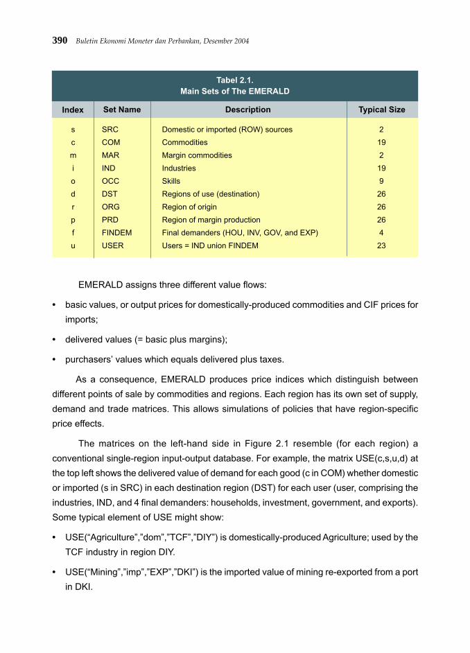
EMERALD assigns three different value flows:
• basic values, or output prices for domestically-produced commodities and CIF prices for
imports;
• delivered values (= basic plus margins);
• purchasers’ values which equals delivered plus taxes.
As a consequence, EMERALD produces price indices which distinguish between
different points of sale by commodities and regions. Each region has its own set of supply,
demand and trade matrices. This allows simulations of policies that have region-specific
price effects.
The matrices on the left-hand side in Figure 2.1 resemble (for each region) a
conventional single-region input-output database. For example, the matrix USE(c,s,u,d) at
the top left shows the delivered value of demand for each good (c in COM) whether domestic
or imported (s in SRC) in each destination region (DST) for each user (user, comprising the
industries, IND, and 4 final demanders: households, investment, government, and exports).
Some typical element of USE might show:
• USE(“Agriculture”,”dom”,”TCF”,”DIY”) is domestically-produced Agriculture; used by the
TCF industry in region DIY.
• USE(“Mining”,”imp”,”EXP”,”DKI”) is the imported value of mining re-exported from a port
in DKI.
Tabel 2.1.Main Sets of The EMERALD
Index Set Name Description Typical Size
s SRC Domestic or imported (ROW) sources 2
c COM Commodities 19
m MAR Margin commodities 2
i IND Industries 19
o OCC Skills 9
d DST Regions of use (destination) 26
r ORG Region of origin 26
p PRD Region of margin production 26
f FINDEM Final demanders (HOU, INV, GOV, and EXP) 4
u USER Users = IND union FINDEM 23

391Illustrative Subsidy Variations to Attract Investors
As the last example shows, the data structure allows for re-export (at least in principle).
All these USE values are “delivered”: they include the value of any trade or transport margins
used to bring goods to the user. Notice also that the USE matrix contains no information
about the regional sourcing of goods.
The TAX matrix of commodity tax revenues contains an element corresponding to
each element of USE. Together with matrices of primary factor cost and production taxes,
these add up to the cost of production (or value of output) of each regional industry.
In principle, each industry is capable of producing any good. The MAKE matrix at the
bottom of Figure 2.1 shows the value of output of each commodity by each industry in each
region d.
EMERALD recognises inventory changes in a limited way. First, changes in stocks of
imports are ignored. For domestic output, stocks are unsold industry outputs, so the dimension
of stocks is STOCK (i,d) rather than STOCK(c,d).
USE(c,s,u,d) is the delivered value of commodity c from source s used by users u in
region d. Delivered value means basic plus margin values. To produce USE(c,s,u,d) from
the DELIVRD(c,s,r,d), EMERALD assumes that all users of a given good (c,s) in a given
region (d) have the same sourcing (r) mix. In effect, for each good (c,s) and region of use (d)
there is a broker who decides for all users in d from which source region, r, supplies will be
obtained. We use the Armington (1969, 1970) sourcing assumption that DELIVRD_R (c,s,d)
is a CES composite (over r in ORG) of the DELIVRD(c,s,r,d).
The DELIVRD(c,s,r,d) matrix shows the delivered value of demand of commodity c,
source s, from region r to region d. For each flow there is a quantity and a price variable. For
example, pdeliverd(c,s,r,d) and xtrad(c,s,r,d) are price and quantity variables corresponding
to the matrix DELIVRD(c,s,r,d).
Using a CES nest, the quantity of goods from different regions of r to destination d,
xtrad(c,s,r,d), is proportional to the quantity of goods summed over r, xtrad_r(c,s,d) and to a
price term powered by elasticities of substitution, SIGMADOMDOM(c), between the source
regions for each commodity c. The price term is composed of relative price, pdeliverd(c,s,r,d)
to puse(c,s,d). Changes in the relative prices of commodity between r induce substitution in
favour of relatively cheapening goods.
Because DELIVRD(c,s,r,d) is comprised of TRADE(c,s,r,d) plus sum{m,MAR,
TRADMAR (c,s,m,r,d)}, we used xtrad(c,s,r,d) as a quantity variable for both DELIVRD(c,s,r,d)
and TRADE(c,s,r,d). The delivered prices variable, pdelivrd(c,s,r,d), is used for
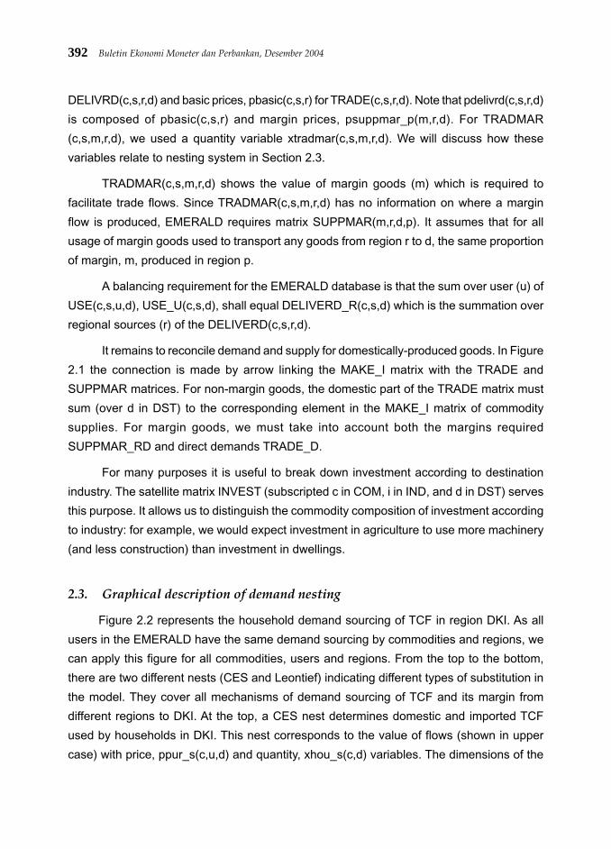
392 Buletin Ekonomi Moneter dan Perbankan, Desember 2004
DELIVRD(c,s,r,d) and basic prices, pbasic(c,s,r) for TRADE(c,s,r,d). Note that pdelivrd(c,s,r,d)
is composed of pbasic(c,s,r) and margin prices, psuppmar_p(m,r,d). For TRADMAR
(c,s,m,r,d), we used a quantity variable xtradmar(c,s,m,r,d). We will discuss how these
variables relate to nesting system in Section 2.3.
TRADMAR(c,s,m,r,d) shows the value of margin goods (m) which is required to
facilitate trade flows. Since TRADMAR(c,s,m,r,d) has no information on where a margin
flow is produced, EMERALD requires matrix SUPPMAR(m,r,d,p). It assumes that for all
usage of margin goods used to transport any goods from region r to d, the same proportion
of margin, m, produced in region p.
A balancing requirement for the EMERALD database is that the sum over user (u) of
USE(c,s,u,d), USE_U(c,s,d), shall equal DELIVERD_R(c,s,d) which is the summation over
regional sources (r) of the DELIVERD(c,s,r,d).
It remains to reconcile demand and supply for domestically-produced goods. In Figure
2.1 the connection is made by arrow linking the MAKE_I matrix with the TRADE and
SUPPMAR matrices. For non-margin goods, the domestic part of the TRADE matrix must
sum (over d in DST) to the corresponding element in the MAKE_I matrix of commodity
supplies. For margin goods, we must take into account both the margins required
SUPPMAR_RD and direct demands TRADE_D.
For many purposes it is useful to break down investment according to destination
industry. The satellite matrix INVEST (subscripted c in COM, i in IND, and d in DST) serves
this purpose. It allows us to distinguish the commodity composition of investment according
to industry: for example, we would expect investment in agriculture to use more machinery
(and less construction) than investment in dwellings.
2.3. Graphical description of demand nesting
Figure 2.2 represents the household demand sourcing of TCF in region DKI. As all
users in the EMERALD have the same demand sourcing by commodities and regions, we
can apply this figure for all commodities, users and regions. From the top to the bottom,
there are two different nests (CES and Leontief) indicating different types of substitution in
the model. They cover all mechanisms of demand sourcing of TCF and its margin from
different regions to DKI. At the top, a CES nest determines domestic and imported TCF
used by households in DKI. This nest corresponds to the value of flows (shown in upper
case) with price, ppur_s(c,u,d) and quantity, xhou_s(c,d) variables. The dimensions of the

393Illustrative Subsidy Variations to Attract Investors
model correspond to the matrices in Figure 2.1. Note that these flows are purchasers values
which are the sum of USE(c,s,u,d) and TAX(c,s,u,d) matrices. The Armington elasticity 2.6
represents a CES in choosing between imported (from other country) and domestic TCF.
Figure 2.1The EMERALD flows Database
USER x DST
IND
USE
(c,s,u,d)
Delivered value of demands:
basic + margins (ex_tax)
quantity: xint(c,s,i,d)
price: puse(c,s,d)
INVEST (c,i,d)purchasers value of good c usedfor investment in industry i in d
price: pinvest (c,d)quantity: xinvi(c,i,d)
TAX
(c,s,u,d)
Commodity taxes
COM
x SRC
FACTORS
LAB (i,o,d) labour
CAP (i,d) capital rental
LND (i,d) land rentals
PRODTAX (i,d) production tax
+
+
=
=
MAKE
(c,i,d)
output of good c by industry i in d
update: xmake(c,i,d)*pdom(c,d)
IND x DST
+
COM
= =
DST
CES
ORG x DST
DELIVRD
(c,s,r,d)
= TRADE(c,s,r,d)
+ sum{m,MAR, TRADMAR(c,s,m,r,d)}
price: pdelivrd(c,s,r,d)
quantity: xtrad(c,s,r,d)
=
TRADE(c,s,r,d)
goods c, s, from r to d at basic pricesprice: pbasic(c,s,r)
quantity: xtrad(c,s,r,d)
TRADMAR
(c,s,m,r,d)
margin m on good c, s from r to d
price: psuppmar_p(m,r,d)
quantity: xtradmar(c,s,m,r,d)
SUPPMAR(m,r,d,p)
Margins supplied by p on goods passingfrom r to d
update:xsuppmar(m,r,d,p) * pdom(m,p)
MAKE_I(m,p)=SUPPMAR_RD(m,p) +TRADE_D(m,"dom",p)
TRADMAR_CS(m,r,d)
SUPPMAR_P(m,r,d)
CES sum over p in REGPRD
sum over COM and SRC
=sum over
i in IND
MAKE_I(c,r)
=TRADE_D
(c,"dom",r)
=
= Leontief
+
INDUSTRY OUTPUT:VTOT(i,d)
INVENTORIES: STOCKS (i,d)
DST ORG x DST
INDEX Set Description
c COM Commoditiess SRC Domestic or imported (ROW) sources
m MAR Margin commodities
r ORG Region of origind DST Region of use (destination)
p PRD Region of margin productionf FINDEM Final demanders (HOU, INV, GOV, EXP)
i IND Industriesu USER Users = IND union FINDEM
IMPORT
(c,r)
USE_U(c,s,d)
=DELIVRD_
R(c,s,d)
price:pdelivrd_r
(c,s,d)
FINDEM(HOU, INV,
GOV, EXP)final demands
by 4 users atdelivered price:
puse(c,s,d)quantities:
xhou(c,s,d)xinv(c,s,d)
xgov(c,s,d)xexp(c,s,d)
COM
x SRC
MAKE_I(c,d)
domestic
commoditysupplies
(c,s,d)

394 Buletin Ekonomi Moneter dan Perbankan, Desember 2004
Demand for domestic TCF in DKI is summed over users to give total value
USE_U(c,s,d) which is measured in delivered value (basic plus margin but excluding user-
specific commodity taxes). Note that this nest is not user-specific. This nest represents
demand for domestic TCF in DKI supplied by all origin of TCF. The CES determines the
allocations with substitution elasticities ranging from 5 (merchandise) to 0.2 (services).
This CES implies that the region with lowered production costs compared to other regions
will tend to increase its market share. The sourcing decision is made on the basis of
delivered prices so not only basic costs affect regional market share but also margin
costs. Note that variables in this nest lack a user (u) subscript. The decision is made on an
all-user basis. The implication is that, in DKI, the proportion of TCF which come from
JaTeng is the same for all users.
The next level indicates how a “delivered” TCF from JaTeng is a Leontief composite
of basic TCF, corresponding with matrix TRADE(c,s,r,d), and the various margin goods,
TRADMAR (c,s,m,r,d). The share of each margin in the delivered price is specific to a particular
combination of origin, destination, commodity and source. For example, we should expect
transport costs to form a larger share for region pairs which are far apart, or for heavy or
bulky goods. The number of margin goods will depend on how aggregated is the model
database. Under the Leontief specification we prevent substitution between road and trade
margins.
The bottom part shows that the margin on TCF passing from JaBar to DKI could be
produced in different regions. The figure shows the sourcing mechanism for the road margin.
We might expect this to be drawn more or less equally from origin (JaTeng), the destination
(DKI) and regions between (JaBar). There would be some scope for substitution (s=1),
since trucking firms can relocate depots to cheaper regions. For retail margins, on the other
hand, a larger share would be drawn from destination region, and scope for substitution
would be less (s=0.1). Once again, this substitution decision takes place at an aggregated
level. The assumption is that the share for example, JaBar, in providing road margin on trips
from JaTeng to DKI, is the same whatever good is being transported. This corresponds to
TRADMAR_CS(m,r,d) which has no c and s scripts. Although not shown in Figure 2.2, a
parallel system of sourcing is also modelled for imported TCF, tracing them back to port of
entry instead of region of production.
2.4. Graphical description of production nesting
The EMERALD adapts production nests from ORANI. This allows each industry to

395Illustrative Subsidy Variations to Attract Investors
produce several commodities, using as inputs domestic and imported commodities, labour
of several types, land, capital and ‘other costs’ which are all distinguished by region. The
multi-input, multi-output production specification is kept manageable by a series of
separability assumptions, illustrated by the nesting shown in Figure 2.3. For example, the
assumption of input-output separability implies that the generalised production function
for some industry:
F(inputs, outputs) = 0 (1)
may be written as:
G(inputs) = X1TOT = H(outputs) (2)
where X1TOT is an index of industry activity. Assumptions of this type reduce the
number of estimated parameters required by the model. Figure 2.3 shows that the H
function in (2) is derived from a CET (constant elasticity of transformation) aggregation
function.
The G function is broken into a sequence of nests. At the top level, commodity
composites, a primary-factor composite and production costs are combined using a Leontief
production function.
Consequently, they are all demanded in direct proportion to X1TOT. Each
commodity composite is a CES (constant elasticity of substitution) function of a domestic
good and the imported equivalent. We adopt the Armington (1969; 1970) assumption
that imports are imperfect substitutes for domestic supplies2 . The primary-factor
composite is a CES aggregation of land, capital and composite labour. Composite labour
is a CES aggregation of occupational labour types. Although all industries share this
common production structure, input proportions and behavioural parameters may vary
between industries.
The nested structure is mirrored in the TABLO equations—each nest requiring 2 sets
of equations, determining quantity and price.
2 Armington PS (1969) The Geographic Pattern of Trade and the Effects of Price Changes, IMF Staff Papers, XVI, July, pp176-199.— (1970) Adjustment of Trade Balances: Some Experiments with a Model of Trade Among Many Countries, IMF StaffPapers, XVII, November, pp 488-523.

396 Buletin Ekonomi Moneter dan Perbankan, Desember 2004
Figure 2.2The EMERALD Demand Nesting
USE_U(c,s,d)pdelivrd_r(c,s,d)xtrad_r(c,s,d)
PUR_S(c,u,d)ppur_s(c,u,d)xhou_s(c,d)
TCF to Householdsin DKI
CES
Imported TCF Domestic TCFPUR(c,s,u,d)ppur_s(c,u,d)xhou_s(c,d)
c = "TCF"u = "Hou"d = "DKI"note :DKI = JakartaJaBar = West JavaJaTeng = Central JavaDIY = Yogyakarta
user-specificpurchasers' value
add over users
Domestic TCF
DIYJaBar JaTeng
TCF
TradeRoad
transportWater
transport
DIY
Roadtransport
JaTengJaBar
CES
CES
Leontief
DELIVRD(c,s,r,d)pdelivrd(c,s,r,d)
xtrad(c,s,r,d)
TRADE(c,s,r,d)pbasic(c,s,r)xtrad(c,s,r,d)
TRADMAR(c,s,m,r,d)psuppmar_p(m,r,d)xtradmar(c,s,m,r,d)
TRADMAR(c,s,m,r,d)psuppmar_p(m,r,d)xtradmar(c,s,m,r,d)
SUPPMAR(m,r,d,p)pdom(m,p)
xsuppmar(m,r,d,p)
not user-specificdelivered values
s = 5
s = 2.6
s = 1
originspecificdeliveredprices
origin of TCF
add over sourceand commodities
Region where road margin is produced

397Illustrative Subsidy Variations to Attract Investors
2.5. Computational efficiency
The EMERALD is able to handle a greater number of regions or sectors than previous
multiregional models through key assumptions that compress the database and enhance
computational efficiency. For example, EMERALD assumes that all users (i.e. downstream
industries, households and government) in a particular region of, say, textiles clothing and
footwear (TCF), source their TCF from other regions according to common proportions. By
assuming this, we notice that the model needs two sub-sourcing matrices (Table 2.2):
USE(c,s,u,d) and TRADE(c,s,r,d). By using the typical set sizes shown in Table 2.2, both
sourcing matrices need 48412 cells. Without the common sourcing assumption 590 thousand
numbers would be needed. The EMERALD becomes 12 times more efficient. This efficiency
will be multiplied by the number of margin commodities if we apply
Figure 2.3The EMERALD Production Nesting
CET
Good 1 ----- up to ------
Activity level
Good 1
Good 2 Good C
Good C Primaryfactors
Production tax
Leontief
CES CES
DomesticGood 1
ImportedGood 1
DomesticGood C
ImportedGood C
Land Labour Capital
inputs oroutputs
functionalform
Key CES
Labourtype 1 --up to--
----- up to ----
Labourtype 2
Labourtype 0
CES
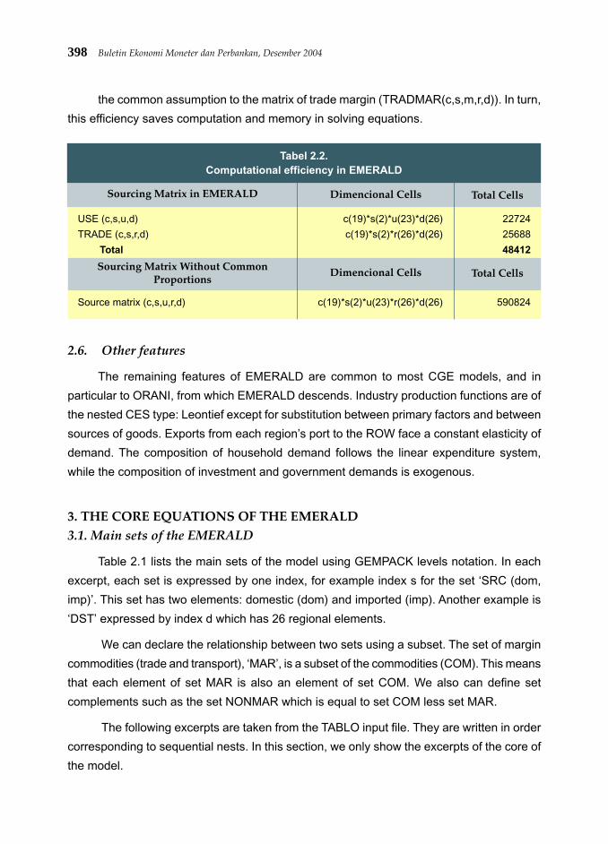
398 Buletin Ekonomi Moneter dan Perbankan, Desember 2004
the common assumption to the matrix of trade margin (TRADMAR(c,s,m,r,d)). In turn,
this efficiency saves computation and memory in solving equations.
Tabel 2.2.Computational efficiency in EMERALD
Dimencional CellsSourcing Matrix in EMERALD Total Cells
USE (c,s,u,d) c(19)*s(2)*u(23)*d(26) 22724
TRADE (c,s,r,d) c(19)*s(2)*r(26)*d(26) 25688
Total 48412
Dimencional CellsSourcing Matrix Without CommonProportions Total Cells
Source matrix (c,s,u,r,d) c(19)*s(2)*u(23)*r(26)*d(26) 590824
2.6. Other features
The remaining features of EMERALD are common to most CGE models, and in
particular to ORANI, from which EMERALD descends. Industry production functions are of
the nested CES type: Leontief except for substitution between primary factors and between
sources of goods. Exports from each region’s port to the ROW face a constant elasticity of
demand. The composition of household demand follows the linear expenditure system,
while the composition of investment and government demands is exogenous.
3. THE CORE EQUATIONS OF THE EMERALD3.1. Main sets of the EMERALD
Table 2.1 lists the main sets of the model using GEMPACK levels notation. In each
excerpt, each set is expressed by one index, for example index s for the set ‘SRC (dom,
imp)’. This set has two elements: domestic (dom) and imported (imp). Another example is
‘DST’ expressed by index d which has 26 regional elements.
We can declare the relationship between two sets using a subset. The set of margin
commodities (trade and transport), ‘MAR’, is a subset of the commodities (COM). This means
that each element of set MAR is also an element of set COM. We also can define set
complements such as the set NONMAR which is equal to set COM less set MAR.
The following excerpts are taken from the TABLO input file. They are written in order
corresponding to sequential nests. In this section, we only show the excerpts of the core of
the model.

399Illustrative Subsidy Variations to Attract Investors
Each excerpt begins with a list of parameters or variables indicated by a name followed
by an index such as ‘(c)’. The expression ‘(c)’ stands for commodities. It signifies that the
variable is a vector containing one value or scalar parameter for each element of the set
commodities, COM. The parameter ‘SIGMADOMIMP(c)’, for example, is the substitution of
elasticity between domestic and imported good by commodity, c.
3.2. Industries choice between domestic and imported goods
Equation 1.1 determines the demand for domestic and imported goods used by
producers in region d. Each industry minimizes cost using a CES (constant elasticity
substitution) nest. Various nest equations follow the same pattern. Each nest includes a
quantity and a price equation.
The intermediate demand for producers, XINT(c,s,i,d), is proportional to overall
composite goods demanded by industry i, XINT_S(c,i,d), and to a price term powered by
the substitution elasticity between domestic and imported goods, SIGMADOMIMP(c). The
price term is the ratio of purchasers’ prices, PPUR(c,s,i,d), to purchasers’ prices averaged
over source, PPUR_S(c,i,d). Changes in relative prices of domestic and imported goods
induce substitution in favour of relatively cheapening goods.
The denominator in the relative price term above is given by Equation 1.2.
Excerpt 1 of TABLO input file: !
! Industries choice between domestic and imported goods !
SIGMADOMIMP(c) Parameter substitution elasticity between dom/imp
BXINT(c,s,i,d) Parameter constant in intermediate demands
XINT(c,s,i,d) Intermediate demands for all-region composite
XINT_S(c,i,d) Industry demands for domestic/imported composite
PPUR(c,s,u,d) User (purchasers) prices, include margins and taxes
PPUR_S(c,u,d) User prices, average over s
(1.1) XINT(c,s,i,d)/XINT_S(c,i,d)= BXINT(c,s,i,d)
*[PPUR(c,s,i,d)/PPUR_S(c,i,d)]**-SIGMADOMIMP(c)
(1.2) PPUR_S(c,i,d)*XINT_S(c,i,d)=sum{s,SRC,PPUR(c,s,i,d)
*XINT(c,s,i,d)}

400 Buletin Ekonomi Moneter dan Perbankan, Desember 2004
3.3. Household choice between domestic and imported goods
Likewise, Equation 2.1 shows that the demand for domestic and imported goods for
household in region d, XHOU(c,s,d), is proportional to overall household composite goods
demand, XHOU_S(c,d), and to a price term powered by the substitution elasticity between
domestic and imported goods, SIGMADOMIMP(c). The price term is the ratio of purchasers’
prices, PPUR(c,s,”hou”,d), to the composite price index, PPUR_S(c,”hou”,d). Again the
denominator PPUR(c,s,”hou”,d) is given by Equation 2.2.
! Excerpt 2 of TABLO input file: !
! Household choice between domestic and imported goods !
BHOU(c,s,d) Parameter: constant in household demands
XHOU(c,s,d) Household demands for all-region composite
XHOU_S(c,d) Household demands for domestic/imported composite
(2.1) XHOU(c,s,d)/XHOU_S(c,d)= BHOU(c,s,d)
*[PPUR(c,s,”HOU”,d)/PPUR_S(c,”hou”,d)]**-SIGMADOMIMP(c)
(2.2) PPUR_S(c,”hou”,d)*XHOU_S(c,d)=sum{s,SRC,PPUR(c,s,”hou”,d)
*XHOU(c,s,d)}
3.4. Investors choice between domestic and imported goods
Equation 3.1 follows the same pattern as previous. It shows that the demand for
domestic and imported goods for investors in region d, XINV(c,s,d), is proportional to overall
investors’ composite goods demand, XINV_S(c,d), and to a price term powered by the
substitution elasticity between domestic and imported goods, SIGMADOMIMP(c). The price
term is the ratio of investment purchasers’ prices to average (over domestic and imported)
prices. The denominator PPUR(c,s,”inv”,d) is given by Equation 3.2
! Excerpt 3 of TABLO input file: !
! Investors choice between domestic and imported goods !
BINV(c,s,d) Parameter constant in investment demands
XINV(c,s,d) Investment demands for all-region composite
XINV_S(c,d) Investment demands for domestic/imported composite

401Illustrative Subsidy Variations to Attract Investors
(3.1) XINV(c,s,d)/XINV_S(c,d) = BINV(c,s,d)
*[PPUR(c,s,”INV”,d)/PPUR_S(c,”inv”,d)]**-SIGMADOMIMP(c)
(3.2) PPUR_S(c,”inv”,d)*XINV_S(c,d) = sum{s,SRC,PPUR(c,s,”inv”,d)
*XINV(c,s,d)}
3.5. Labour skill nest
Excerpt 4 represents a labour skill nest to minimize labour cost. Similar with the
previous, this nest is expressed by Equation 4.1 determining labour demand of industry i for
different occupations, XLAB(i,o,d). The average industry wage, PLAB_O(i,d), is determined
by Equation 4.2.
! Excerpt 4 of TABLO input file: !
! Labour skill nest !
SIGMALAB(i) Parameter CES substitution between skill types
BLAB(i,o,d) Parameter constant in labour demand equation
XLAB(i,o,d) Labour demands
XLAB_O(i,d) Effective labour input
PLAB(i,o,d) Wage rates
PLAB_O(i,d) Price of labour composite
(4.1) XLAB(i,o,d)/XLAB_O(i,d) = BLAB(i,o,d)
*[PLAB(i,o,d)/PLAB_O(i,d)]**-SIGMALAB(i)
(4.2) PLAB_O(i,d)*XLAB_O(i,d) = sum{o,OCC,PLAB(i,o,d)* XLAB(i,o,d)}
The XLAB(i,o,d) is proportional to effective labour input, XLAB_O(i,d), and to a wage
term powered by elasticities of substitution between labour skill in each industry,
SIGMALAB(i). The wage term is ratio of wage rates, PLAB(i,o,d), to price of labour composite,
PLAB_O(i,d). Changes in relative occupational wages induce substitution in favour of
relatively cheaper skills.
3.6. Demands for primary factors
Excerpt 5 explains demands for primary factors. The effective labour, capital, and

402 Buletin Ekonomi Moneter dan Perbankan, Desember 2004
land cost are combined using a CES nest. Ignoring the labour technological change terms,
ALAB_O(i,d), the effective labour demand, XLAB_O, is proportional to overall primary factor
demands, XPRIM(i,d), and to a price term powered by the elasticity of substitution between
primary factors, SIGMAPRIM (i). The price term is the relative price of the labour composite,
PLAB_O(i,d), to the price of composite factors, PPRIM(i,d). Changes in the price term induce
substitution in favour of relatively cheapening factors. The same rules govern for capital and
land demand.
The price of factor composite, PPRIM(i,d), is determined by the value of the primary
factor composite equalling the sum of all component costs.
! Excerpt 5 of TABLO input file: !
! Demands for primary factors !
SIGMAPRIM(i) Parameter CES substitution, primary factors
BLAB_O(i,d) Parameter constant in effective labour demand
BCAP(i,d) Parameter constant in capital demand equation
BLND(i,d) Parameter constant in land demand equation
ACAP(i,d) Capital usage technological change
ALAB_O(i,d) Effective labour input technological change
ALND(i,d) Land usage technological change
XCAP(i,d) Capital usage
XLND(i,d) Land usage
XPRIM (i,d) Effective composite inputs
PCAP(i,d) Rental price of capital
PLND(i,d) Rental price of land
PPRIM(i,d) Price of factor composite
(5.1) XLAB_O(i,d)/[XPRIM(i,d)*ALAB_O(i,d)]=BLAB_O(i,d)
*[[PLAB_O(i,d)*ALAB_O(i,d)]/PPRIM(i,d)]**-SIGMAPRIM(i)
(5.2) XCAP(i,d)/[XPRIM(i,d)*ACAP(i,d)]=BCAP(i,d)
*[[PCAP(i,d)*ACAP(i,d)]/PPRIM(i,d)]**-SIGMAPRIM(i)

403Illustrative Subsidy Variations to Attract Investors
(5.3) XLND(i,d)/[XPRIM(i,d)*ALND(i,d)]=BLND(i,d)
*[[PLND(i,d)*ALND(i,d)]/PPRIM(i,d)]**-SIGMAPRIM(i)
(5.4) PPRIM(i,d)*XPRIM(i,d)=PLAB_O(i,d)*XLAB_O(i,d)
+PCAP(i,d)*XCAP(i,d)+PLND(i,d)*XLND(i,d)
3.7. Demands for aggregate primary factors and intermediate inputs
For the top nest, excerpt 6 explains how to produce output using a combination of
composite primary inputs, XPRIM(i,d), and composite intermediate goods, XINT_S(c,i,d),
with Leontief elasticity of substitution. As a consequence, the demand equations for
XPRIM(i,d) and XINT_S(c,i,d) have a similar pattern as seen in two equations below.
Equation 6.1 explains that the industry demand for aggregate primary factor,
XPRIM(i,d), is proportional to total output and technological terms. Equation 6.2 explains
that the demand for composite goods, XINT_S(c,i,d) is also proportional to total output and
technological terms. We recognise three different technological terms, APRIM(i,d),
AINT_S(c,i,d) and ATOT(i,d). Technological change implies change in input requirement
per unit of output. When these technological terms reduce, the same level of output is
produced using less XPRIM(i,d) or XINT_S(c,i,d).
The third equation, Equation 6.3 is the ‘Zero Pure Profits’. Total revenue is equal to
total cost of all inputs.
! Excerpt 6 of TABLO input file: !
! Demands for aggregate primary factor and intermediate inputs !
APRIM(i,d) Primary inputs technological change
AINT_S(c,i,d) Intermediate composite technological change
ATOT(i,d) Industry output technological change
XTOT(i,d) Industry outputs
PCST(i,d) Production cost
(6.1) XPRIM(i,d) = APRIM(i,d)*ATOT(i,d)*XTOT(i,d)
(6.2) XINT_S(c,i,d) = AINT_S(c,i,d)*ATOT(i,d)*XTOT(i,d)
(6.3) PCST(i,d)*XTOT(i,d) = sum{c,COM,PPUR_S(c,i,d)*XINT_S(c,i,d)}

404 Buletin Ekonomi Moneter dan Perbankan, Desember 2004
+sum{o,OCC,PLAB(i,o,d)*XLAB(i,o,d)}
+PCAP(i,d)*XCAP(i,d)+PLND(i,d)*XLND(i,d)
3.8. Adding production tax to firm costs
Excerpt 7 explains how a production tax is added to the firm cost. Equation 7.1 indicates
that a change in production tax revenue, PTX(i,d), is determined by change in PTXRATE(i,d)
multiplied by the value of output, (PCST(i,d)*XTOT(i,d)).
Equation 7.2 sets industry output price, PTOT(i,d), via the firm cost, PCST(i) and the
tax revenue PTX(i,d).
! Excerpt 7 of TABLO input file: !
! Adding Production tax to firm costs !
PTOT(i,d) Industry output prices
PTXRATE(i,d) Rate of production tax
PTX(i,d) Ordinary change in production tax revenue
(7.1) PTX(i,d) = PTXRATE(i,d)*PCST(i,d)*XTOT(i,d)
(7.2) PTOT(i,d)*XTOT(i,d) = PCST(i,d)*XTOT(i,d)+PTX(i,d)
3.9. MAKE: multi-product industries have CET specification
Equation 8.1 explains supplies of commodities by industries, XMAKE(c,i,d), with
constant elasticity transformation (CET). Ignoring the technological term, AMAKE(c,i,d), output
each commodity supplied by an industry, XMAKE(c,i,d), is proportional to XTOT (i,d) and to
a price term powered by SIGMAOUT (i). The price term is composed of the price of domestic
good relative to average price of industry i output. Since SIGMAOUT (i) is positive, this
induces industries to produce more of the commodity with an increased relative prices.
Equation 8.2 equates the output value of industry (PTOT(i,d)*XTOT(i,d) equals to the
sum of commodities supplied by industry calculated using domestic prices, PDOM(c,d).
Equation 8.3 shows that total output of commodities, XCOM(c,d), is equal to the sum
of commodities supplied by various industries.
Lastly, import prices, PIMP(c,r), in Equation 8.4, are simply determined by foreign
import prices, PFIMP(c,r) multiplied by the exchange rate, PHI.

405Illustrative Subsidy Variations to Attract Investors
! Excerpt 8 of TABLO input file: !
! MAKE: multi-product industries have CET specification !
SIGMAOUT(i) Parameter CET transformation elasticities
AMAKE(c,i,d) MAKE technological change
XMAKE(c,i,d) Output of good c by industry i in d
XCOM(c,d) Total output of commodities
PDOM(c,r) Output prices = basic prices of domestic goods
PFIMP(c,r) Import prices, foreign currency
PIMP(c,r) Import prices, local currency
PHI Exchange rate
(8.1) XMAKE(c,i,d) = AMAKE(c,i,d)*XTOT(i,d)*
{[PDOM(c,d)/PTOT(i,d)]**SIGMAOUT(i)}
(8.2) PTOT(i,d)*XTOT(i,d) = sum{c,COM,PDOM(c,d)* XMAKE(c,i,d)}
(8.3) XCOM(c,d) = sum{i,IND, XMAKE(c,i,d)}
(8.4) PIMP(c,r) = PFIMP(c,r)*PHI
3.10. Household demands
Excerpt 9 determines the allocation of household expenditure between commodity
composites. This is derived from the Klein-Rubin utility function:
Utility per household = P {X3_S(c) -
X3SUB(c)}S3LUX(c),
The X3SUB and S3LUX are behavioural coefficients—the S3LUX must sum to unity. Q
is the number of households. The demand equations that arise from this utility function are:
X3_S(c) = X3SUB(c) + S3LUX(c)*V3LUX_C/P3_S(c),
where:
V3LUX_C = V3TOT - ÂX3SUB(c)* P3_S(c)
The name of the linear expenditure system derives from its property that expenditure
on each good is a linear function of prices (P3_S) and expenditure (V3TOT). The form of the
demand equations gives rise to the following interpretation. The X3SUB are said to be the

406 Buletin Ekonomi Moneter dan Perbankan, Desember 2004
‘subsistence’ requirements of each good—these quantities are purchased regardless of
price. V3LUX_C is what remains of the consumer budget after subsistence expenditures
are deducted—we call this ‘luxury’ or ‘supernumerary’ expenditure. The S3LUX are the
shares of this remnant allocated to each good—the marginal budget shares.
The simplicity of this scheme is that LES has no specific substitutability. Hence, LES
requires only a vector of expenditure elasticities and 1 Frisch parameter for each region.
Equation 9.1, an alias, equates household prices by commodity, PHOU(c,d), to the
household purchasing prices, PPUR_S(c,”hou”,d). Household subsistence costs in d,
WSUBSIST(d), are defined by Equation 9.2 as total per capita subsistence expenditure
spent by the number of households NHOU(d). The household expenditure is composed by
consumer prices, PHOU(c,d), multiplied by household subsistence quantities,
XSUBSIST(c,d).
Equation 9.3 determines that total household demand for composite commodities,
XHOU_S(c,d), is proportional to marginal budget share, MBS(c,d) multiplied by luxury cost.
The luxury cost is household purchasing value other than subsistence cost, (WHOUTOT(d)-
WSUBSIST(d)). Then, the nominal household expenditure, WHOUTOT(d) is PHOUTOT(d)
multiplied by total household expenditure, XHOUTOT(d).
Equation 9.4 determines that budget share, BUDGSHR(c,d), is the ratio of household
purchasing value to total nominal household consumption.
Equation 9.5 determines PHOUTOT (d), as consumer price index, which is the sum
over consumer price by commodity, PHOU(c,d), multiplied by budget share, BUDGSHR(c,d).
Since WHOUTOT(d) and PHOUTOT(d) are known, total real household consumption,
XHOUTOT(d) and WHOUTOT(d) are given by Equation 9.6 and Equation 9.7.
! Excerpt 9 of TABLO input file: !
! Household demands !
MBS(c,d) Parameter marginal budget shares
BUDGSHR(c,d) Average budget shares
WHOUTOT(d) Total nominal household consumption
WSUBSIST(d) Household subsistence costs
XHOUTOT(d) Total real household consumption
PHOUTOT(d) CPI

407Illustrative Subsidy Variations to Attract Investors
NHOU(d) Number of households
XSUBSIST(c,d) Household subsistence quantities
PHOU(c,d) Household price of composites
(9.1) PHOU(c,d)= PPUR_S(c,”hou”,d)
(9.2) WSUBSIST(d)= sum{c,COM,PHOU(c,d)*NHOU(d)*XSUBSIST(c,d)}
(9.3) XHOU_S(c,d)*PHOU(c,d) = MBS(c,d)*[WHOUTOT(d) - WSUBSIST(d)]
(9.4) BUDGSHR(c,d) = PUR_S(c,”Hou”,d)/WHOUTOT(d)
(9.5) PHOUTOT(d)= sum{c,COM,BUDGSHR(c,d)*PHOU(c,d)}
(9.6) XHOUTOT(d)= WHOUTOT(d)/PHOUTOT(d)
(9.7) WHOUTOT(d)= PHOUTOT(d) * XHOUTOT(d)
3.11. Investment demands and indices: conditional on industry-specificinvestment
Excerpt 10 shows the equations determining investment demands and indices æ
conditional on industry-specific investment. The equation determining new capital creation
is derived using Leontief technology demand. Equation 10.1 explains that the amount of
good c for investment industry i in d, XINVI(c,i,d) is proportional to investment by industries
in d, XINVITOT(i,d), multiplied by investment technological term, AINVI(c,i,d).
Equation 10.2 defines purchaser’s price of good c for investment in d, PINVEST(c,d)
as investor purchasing price, PPUR_S(c,”INV”,d)
Equation 10.3 determines the investment price index for industry i, in region d,
PINVITOT(i,d) by making an identity between the value of investment by industry i in d as
the sum over commodities used by that industry for investment in d.
Equation 10.4 explains that XINV_S(c,d) is sum over industry demands for investment
goods, XINVI(c,i,d).
! Excerpt 10 of TABLO input file: !
! Investment demands and indices:conditional on industry-specific !
! investment !
AINVI(c,i,d) Investment technological change

408 Buletin Ekonomi Moneter dan Perbankan, Desember 2004
XINVI(c,i,d) Amount of good c for investment, industry i in d
XINVITOT(i,d) Investment by industry
PINVITOT(i,d) Investment price index by industry
PINVEST(c,d) Purchaser’s price of good c for investment in d
(10.1) XINVI(c,i,d) = AINVI(c,i,d)*XINVITOT(i,d)
(10.2) PINVEST(c,d) = PPUR_S(c,”INV”,d)
(10.3) PINVITOT(i,d)*XINVITOT(i,d) = sum{c,COM, PINVEST(c,d)
*XINVI(c,i,d)}
(10.4) XINV_S(c,d)= sum{i,IND,XINVI(c,i,d)}
3.12. Government, export, and inventory demands
Excerpt 11 explains government, export, and inventory demands. As expressed by
Equation 11.1, the government demand is proportional to three corresponding shifters. They
shift the demand function with different dimensions: by d as FGOVTOT(d), by c and d, as
FGOV_S(c,d) and by c, s, and d, as FGOV(c,s,d).
Equation 11.2 explains that demand for export goods, XEXP(c,s,d), is proportional to
export-quantity shifter, FQEXP(c,s) multiplied by a price term powered by export elasticity
substitution, EXP_ELAST(c). The price term is composed of purchasing export prices,
PPUR(c,s,”EXP”,d), relative to the ratio of export price shifter, FPEXP(c,s), and exchange
rate, PHI.
Equation 11.3 defines that stocks, XSTOCKS(i,d), is proportional to XTOT(i,d)
multiplied by stocks shifter, FSTOCKS(i,d).\c AnsiText \* MERGEFORMAT
! Excerpt 11 of TABLO input file: !
! Government, export, and inventory demands !
! Governments !
FGOVTOT(d) Government demand shifter
FGOV(c,s,d) Government demand shifter
FGOV_S(c,d) Government demand shifter
XGOV(c,s,d) Government demand

409Illustrative Subsidy Variations to Attract Investors
(11.1) XGOV(c,s,d) = FGOVTOT(d)*FGOV(c,s,d)*FGOV_S(c,d)
! Exports !
EXP_ELAST(c) Export demand elasticities
FQEXP(c,s) Export quantity shift variable
FPEXP(c,s) Export price shift variable
XEXP(c,s,d) Export of all-region composite leaving port at d
(11.2) XEXP(c,s,d)/FQEXP(c,s)=[PPUR(c,s,”EXP”,d)/
[FPEXP(c,s)/PHI]]**-EXP_ELAST(c)
! Inventories !
FSTOCKS(i,d) Stocks shifter
XSTOCKS(i,d) Inventories
(11.3) XSTOCKS(i,d) = FSTOCKS(i,d)*XTOT(i,d)
3.13. Add up user demands to get total regional demand for delivered goods
Excerpts 12 explains that total regional demand for delivered goods composite c, s in
d, XTRAD_R(c,s,d), is an add up of user demand.
! Excerpt 12 of TABLO input file: !
! Add up user demands to get total regional demand for !
! delivered goods !
XTRAD_R(c,s,d) Total demand for regional composite c,s in d
(12.1) XTRAD_R(c,s,d) = sum{i,IND, XINT(c,s,i,d)}+ XHOU(c,s,d)
+ XINV(c,s,d)+ XGOV(c,s,d)+ XEXP(c,s,d)
3.14. Delivering goods to regions
Excerpt 13 explains delivering goods to regions. Using the Leontief function, Equation
13.1 determines that the demand for margin, XTRADMAR(c,s,m,r,d), is a proportion of XTRAD
(c,s,r,d) multiplied by margin technological term, ATRADMAR(c,s,m,r,d). This
XTRADMAR(c,s,m,r,d) contains a margin flow to facilitate commodities from region r to d.

410 Buletin Ekonomi Moneter dan Perbankan, Desember 2004
The delivered price of good c, s from r to d, PDELIVRD(c,s,r,d) is determined using
Equation 13.2. Since XTRAD(c,s,r,d) is known, the delivered value of commodity c, s, from
r to d (on the left hand side) is composed by the basic plus the margin value used.
! Excerpt 13 of TABLO input file: !
! Delivering goods to regions !
ATRADMAR(c,s,m,r,d) Trade for margins technological change
XTRAD(c,s,r,d) Quantity of good c,s from r to d
XTRADMAR(c,s,m,r,d) Margin m on good c,s going from r to d
PBASIC(c,s,r) Basic prices
PDELIVRD(c,s,r,d) All-user deliverd price of good c,s from r to d
XSUPPMAR_P(m,r,d) Quantity of composite margin m on goods from r to d
PSUPPMAR_P(m,r,d) Price of composite margin m on goods from r to d
(13.1) XTRADMAR(c,s,m,r,d) = ATRADMAR(c,s,m,r,d)* XTRAD(c,s,r,d)
(13.2) PDELIVRD(c,s,r,d)*XTRAD(c,s,r,d) =PBASIC(c,s,r)*XTRAD(c,s,r,d)
+sum{m,MAR, PSUPPMAR_P(m,r,d)*XTRADMAR(c,s,m,r,d)}
3.15 Regional sourcing
For each good and destination region, an average user chooses region sourcing based
on delivered (margin-paid, but ex-tax) prices and values.
Equation 14.1 explains the delivered price of regional composite good c, s, to d,
PUSE(c,s,d). By multiplying PUSE(c,s,d) to XTRAD_R(c,s,d), it converts the left hand side
equation into a value. Since the value of total components on the right hand side and
XTRAD_R(c,s,d) are known, we can determine PUSE(c,s,d).
Equation 14.2 determines the demand of good c, either domestic or imported (s) from
regional source (r) to destination region (d), XTRAD(c,s,r,d) by multiplying XTRAD_R(c,s,d)
to trading share, STRAD(c,s,r,d), and by a price term. The XTRAD_R(c,s,d) is the demand
of good c, s to d sum over region of origins, r. The price term is composed of the ratio
PDELIVRD(c,s,r,d) to PUSE(c,s,d) powered by constant elasticity substitution between region,
SIGMADOMDOM(c), to total good from original regions.

411Illustrative Subsidy Variations to Attract Investors
! Excerpt 14 of TABLO input file: !
! For each good and destination region,an average user chooses !
! regional sourcing !
! Based on delivered (margin-paid, but ex-tax) prices and values !
SIGMADOMDOM(c) Parameter substitution elasticity between origins
PUSE(c,s,d) Delivered price of reg composite good c,s to d
STRAD(c,s,r,d) Initial share
(14.1) PUSE(c,s,d)*XTRAD_R(c,s,d)=sum{r,ORG,PDELIVRD(c,s,r,d)
*XTRAD(c,s,r,d)}
(14.2) XTRAD(c,s,r,d) = STRAD(c,s,r,d)*XTRAD_R(c,s,d)
*[PDELIVRD(c,s,r,d)/PUSE(c,s,d)]**-SIGMADOMDOM(c)
3.16. Where margins are produced
Equation 15.1 contains equations determining where margins are produced. It shows
that the composite margin m on goods passing from r to d, XSUPPMAR_P(m,r,d), is sum
over commodity and source of margin m on good c, s going from r to d, XTRADMAR(c,s,m,r,d).
The price of composite margin m on goods from r to d, PSUPPMAR_P(m,r,d) is given
by Equation 15.2.
Margin m supplied by p on goods passing from r to d, XSUPPMAR(m,r,d,p) as
expressed by Equation 15.3, is proportional to XSUPPMAR_P(m,r,d) multiplied by a price
term. The price term is a ratio PDOM(m,p) to PSUPPMAR_P(m,r,d) powered by substitution
elasticity between margin origins, SIGMAMAR(m).
Adding up total demand for margins produced in p can be expressed into two different
ways, Equation 15.4 and Equation 15.5. One is a sum over d and the other is sum over r
and d.
! Excerpt 15 of TABLO input file: !
! Where margins are produced !
! We need xsuppmar_p(m,r,d) margins !
! What regions p shall they come from ? !

412 Buletin Ekonomi Moneter dan Perbankan, Desember 2004
SIGMAMAR(m) Parameter substitution elast betwen marg origins
BSUPPMAR(m,r,d,p) Parameter:const in demand for marg m (made in p)
XSUPPMAR(m,r,d,p) Demand for marg m (made in p) on goods from r to d
XSUPPMAR_D(m,r,p) Total margins on goods from r, produced in p
XSUPPMAR_RD(m,p) Total demand for margins produced in p
(15.1) XSUPPMAR_P(m,r,d) = sum{c,COM, sum{s,SRC, XTRADMAR(c,s,m,r,d)}}
(15.2) XSUPPMAR_P(m,r,d)*PSUPPMAR_P(m,r,d) =
sum{p,PRD, XSUPPMAR(m,r,d,p)*PDOM(m,p)}
(15.3) XSUPPMAR(m,r,d,p) = BSUPPMAR(m,r,d,p) * XSUPPMAR_P(m,r,d)
*[PDOM(m,p)/PSUPPMAR_P(m,r,d)]**- SIGMAMAR(m)
! Add up total demand for margins produced in p !
(15.4) XSUPPMAR_D(m,r,p) = sum{d,DST, XSUPPMAR(m,r,d,p)}
(15.5) XSUPPMAR_RD(m,p) = sum{r,ORG, XSUPPMAR_D(m,r,p)}
3.17. Total demand for commodity c made in r = supply commodity c made in r
Equation 16.1 explains total demand for commodity c produced in r equal to supply
commodity c, s produced in r.
Specifically for domestic source, TOTDEM(c,”dom”,r) expressed by Equation 16.2, is
equal to supply for non-margins, XCOM(c,r). Then, supply for margins, XCOM(m,p)
determined by Equation 16.3, is composed of direct demands for goods produced
domestically in r, TOTDEM(m,”dom”,p) plus demand for margins produced in p,
XSUPPMAR_RD(m,p).
Equation 16.4 shows that PBASIC(c,”dom”,r) is identical to PDOM(c,r). Equation 16.5
shows that PBASIC(c,”imp”,r) is identical to import price, PIMP(c,r). PPUR(c,s,u,d) is given
by Equation 16.6.
Using Equation 16.7, commodity tax revenue, COMTAXREV(d), is obtained from
total value of goods used by users multiplied by commodity tax rate. Where commodity tax
rate is TAX(c,s,u,d)/USE(c,s,u,d) or [TUSER(c,s,i,d)-1] .

413Illustrative Subsidy Variations to Attract Investors
! Excerpt 16 of TABLO input file: !
! Total demand for commodity c made in r = supply commodity c !
! made in r !
TOTDEM(c,s,r) Total direct demands for goods made and landed in r
TUSER(c,s,u,d) Powers of commodity taxes
COMTAXREV(d) Commodity tax revenue
(16.1) TOTDEM(c,s,r) = sum{d,DST, XTRAD(c,s,r,d)}
(16.2) XCOM(c,r) = TOTDEM(c,”dom”,r)
(16.3) XCOM(m,p) = TOTDEM(m,”dom”,p)+ XSUPPMAR_RD(m,p)
(16.4) PBASIC(c,”dom”,r) = PDOM(c,r)
(16.5) PBASIC(c,”imp”,r) = PIMP(c,r)
(16.6) PPUR(c,s,u,d) = PUSE(c,s,d) * TUSER(c,s,u,d)
(16.7) COMTAXREV(d) = sum{c,COM,sum{s,SRC,
sum{i,IND, [TUSER(c,s,i,d)-1]*PUSE(c,s,d) *XINT(c,s,i,d)}
+[TUSER(c,s,”hou”,d)-1]*PUSE(c,s,d) *XHOU(c,s,d)
+[TUSER(c,s,”gov”,d)-1]*PUSE(c,s,d) *XGOV(c,s,d)
+[TUSER(c,s,”inv”,d)-1]*PUSE(c,s,d) *XINV(c,s,d)
+[TUSER(c,s,”exp”,d)-1]*PUSE(c,s,d) *XEXP(c,s,d)}}
3.18. Industry-specific investment demands
Excerpt 17 describes industry specific investment demands. The gross rate of return,
GRET(i,d), is determined as a ratio of capital rental to price of new capital. The investment
by industries, XINVITOT(i,d) is capital usage, XCAP(i,d), multiplied by the gross growth rate
of capital, GGRO(i,d). Where GGRO(i,d) is determined by the DPSV (Dixon et al. 1982)
investment rule3 .
3 As explained in excerpt 31 of the Oranig03.tab, above equation comes from substituting the values 0.33 and 2.0 whichcorrespond to the DPSV ratios [1/G.Beta] and Q (= ratio, gross to net rate of return) and are typical values of these ratios. InDPSV invslack was called “omega” and was interpreted as the “economy-wide rate of return”.

414 Buletin Ekonomi Moneter dan Perbankan, Desember 2004
! Excerpt 17 of TABLO input file: !
! Industry-specific investment demands !
GRET(i,d) Gross rate of return = rental/[price of new capital]
GGRO(i,d) Gross growth rate of capital = investment/capital
FINV1(i,d) Investment shift variable
INVSLACK Investment slack variable for exogenizing national investment
(17.1) GRET(i,d) = PCAP(i,d) / PINVITOT(i,d)
(17.2) GGRO(i,d)= XINVITOT(i,d) / XCAP(i,d)
(17.3) GGRO(i,d) = FINV1(i,d)*[{GRET(i,d)**2}/INVSLACK]**0.33
The following excerpts are Excerpt 16 and Excerpt 17 but written in percentage changes
version. Equation 16.1 in level version corresponds to Equation 16.1 in the percentage
changes version. We can write an equation in level with several equations in percentages
changes version. For example, Equation 16.7 in level version, it is written by several equations
in percentage changes (from Equation 16.7 to 16.11). Note that we write variable names in
lower case and value flows/coefficients in capital case. Sometimes it is necessary to state a
variable in ordinary change if that variable can change from positive toward negative or
reverse. We write ordinary-change variables with prefix ‘del, for example ‘ delTAXint (c,s,i,d).
This represents ordinary change in TAX for intermediate input demands.
\c AnsiText \* MERGEFORMAT ! Excerpt 16 of TABLO input file: !
! Total demand for commodity c produced in r = supply commodity c !
! produced in r (in percentage changes version) !
! data flows/coefficients !
TRADE(c,s,r,d) Trade matrix (at basic prices)
TRADE_D(c,s,r) Total direct demands
SUPPMAR_RD(m,p) Total demand for margin m produced in p
TAX(c,s,u,d) Commodity taxes
! variables in percentage changes !
totdem(c,s,r) Total direct demand for goods produced(dom)

415Illustrative Subsidy Variations to Attract Investors
orlanded(imp) in r
xtrad(c,s,r,d) Quantity of good c,s from r to d
xcom(c,d) Total output of commodities
ppur(c,s,u,d) User (purchasers) prices, inc margins and taxes
puse(c,s,d) Delivered price of regional composite good c,s to d
tuser(c,s,u,d) Powers of commodity taxes
(16.1) (TRADE_D(c,s,r))*totdem(c,s,r) = sum{d,DST,TRADE(c,s,r,d)
*xtrad(c,s,r,d)}
(16.2) xcom(c,r) = totdem(c,”dom”,r)
(16.3) MAKE_I(m,p)*xcom(m,p) = TRADE_D(m,”dom”,p)*totdem(m,”dom”,p)
+ SUPPMAR_RD(m,p)*xsuppmar_rd(m,p)
(16.4) pbasic(c,”dom”,r) = pdom(c,r)
(16.5) pbasic(c,”imp”,r) = pimp(c,r)
(16.6) ppur(c,s,u,d) = puse(c,s,d) + tuser(c,s,u,d)
! variables in ordinary change !
delTAXint(c,s,i,d) intermediate commodity tax revenue
delTAXhou(c,s,d) household commodity tax revenue
delTAXinv(c,s,d) investment commodity tax revenue
delTAXgov(c,s,d) government commodity tax revenue
delTAXexp(c,s,d) export commodity tax revenue
!variables in percentage changes!
xint(c,s,i,d) Intermediate demands for all-region composite
xhou(c,s,d) Household demands for all-region composite
xinv(c,s,d) Investment demands for all-region composite
xgov(c,s,d) Government demands for all-region composite
xexp(c,s,d) Export of all-region composite leaving port at d

416 Buletin Ekonomi Moneter dan Perbankan, Desember 2004
(16.7) delTAXint(c,s,i,d) = 0.01*TAX(c,s,i,d)
*[xint(c,s,i,d)+puse(c,s,d)] + 0.01*PUR(c,s,i,d)*tuser(c,s,i,d)
(16.8) delTAXhou(c,s,d) = 0.01*TAX(c,s,”hou”,d)
*[xhou(c,s,d)+puse(c,s,d)] + 0.01*PUR(c,s,”hou”,d)*tuser(c,s,”hou”,d)
(16.9) delTAXinv(c,s,d) = 0.01*TAX(c,s,”inv”,d)*[xinv(c,s,d)+puse(c,s,d)]+
0.01*PUR(c,s,”inv”,d)*tuser(c,s,”inv”,d)
(16.10)delTAXgov(c,s,d) = 0.01*TAX(c,s,”gov”,d) *[xgov(c,s,d)+puse(c,s,d)]+
0.01*PUR(c,s,”gov”,d)*tuser(c,s,”gov”,d)
(16.11)delTAXexp(c,s,d) = 0.01*TAX(c,s,”exp”,d)*[xexp(c,s,d)+puse(c,s,d)]+
0.01*PUR(c,s,”exp”,d)*tuser(c,s,”exp”,d)
! Excerpt 17 of TABLO input file: !
! Industry-specific investment demands !
! (in percentage changes version) !
! Variables in percentage changes !
ggro(i,d) Gross growth rate of capital = Investment/capital
gret(i,d) Gross rate of return = Rental/[Price of new capital]
finv1(i,d) Investment shift variable invslack Investment slack for exogenizing
national investment
pcap(i,d) Rental price of capital
pinvitot(i,d) Investment price index by industry
xcap(i,d) Capital usage
xinvitot(i,d) Investment by industry
(17.1) gret(i,d)= pcap(i,d) - pinvitot(i,d)
(17.2) ggro(i,d)= xinvitot(i,d) - xcap(i,d)
(17.3) ggro(i,d) = finv1(i,d) + 0.33*[2.0*gret(i,d) -invslack]

417Illustrative Subsidy Variations to Attract Investors
4. DATABASE4.1. Introduction
Regional input-output tables and trade matrices, as shown in Figure 2.1 Section 2,
are not available in Indonesia. The EMERALD database is produced from very limited regional
data in several steps. Key features of this strategy are:
• The process starts with a national input-output table and certain regional data. The
minimum requirement for regional data is very modest: the distribution between regions
of industry output and of final demand aggregates.
• The database is constructed at the most disaggregated sectoral and regional level: 97
sectors and 26 regions. This is useful when estimating missing data.
The data process is broken into 7 stages, as shown in Figure 4.1:
• A preliminary aggregation to reduce multiproduction
• Simplification of data structure
• Input usage distinguished by place of use
• Input usage distinguished by place of production
• Consolidate final format
• Aggregation into 19 sectors
• Run the model to produce diagnostic information and summary
Our exposition follows these steps.
Remainder of Section 4 omitted to meet size limit. A zip file of the complete section
may be downloaded from http://www.monash.edu.au/policy/archivep.htm.

418 Buletin Ekonomi Moneter dan Perbankan, Desember 2004
Figure 4.1Data Construction
TRADE matrix80 commodity
x [dom,imp] x 26 origin region x 26 dest region
INDOCEEM 200197 sector
HAR database
Data to split usersby 26 dest regionR001 R002 R003
etc
Distance matrix(gravity); importby port of entry
80 sectorINDOCEEM style HAR
database
80 sectorsingle region EMERALD
database
80 sector26 destination database
Stage 1: aggregation
80 sector26 origin 26 dest
EMERALD database
19 sector 26 region
EMERALD database
Data summary and
Diagnostics
demand by region supply
by region
Stage 2: simplify
Stage 3: split users by destination
Stage 4: form trade matrix
Stage 5: consolidate final format
Stage 6:aggregation
Stage 7: run model
data
Key
process

419Illustrative Subsidy Variations to Attract Investors
5. SUBSIDY VARIATIONS TO ATTRACT INVESTORS.5.1. Introduction
This section analyses the economic effects of subsidising industry to attract investment
in specific regions. As an example, we choose to subsidise Textiles, Clothing and Footwear
(TCF) industry in Central Java (JaTeng) using the EMERALD (Equilibrium Model with
Economic Regional AnaLysis Dimensions) multi-regional CGE Model.
We simulate several financial approaches to the TCF subsidy in JaTeng: unfunded
subsidy, subsidy funded by consumer tax or by producer tax, and reduction in local
government demand. Selected results are shown for the target region (JaTeng), a neighbour
region (Yogyakarta) and for the nation. Also we decompose total results into different effects.
For example, we split the total effect of a subsidy funded by consumers into two separate
effects: the effects of the subsidy and the effects of the consumer tax.
5.2. Textile clothing and footwear in JaTeng (Central Java)
Tables 5.1 and 5.2 are examples of data generated for this model. Table 5.1 shows
destinations of TCF made in JaTeng. 26% remains in JaTeng (14% used by industries and
12% by households), other regions take 51% and exports take 22%.
Tabel 5.1.Destinations of TCF made in JaTeng (in billions of Rupiah)
Local (JaTeng)
Intermediate Households Investment GovernmentOther
RegionsROW
ExportTotal
2640 2182 4 8 9356 4055 18245
14.47% 11.96% 0.02% 0.04% 51.28% 22.23% 100%
Table 5.2 shows trade inflows to JaTeng. There are three sources of TCF used in
JaTeng: local (47%), other regions (45%) and import (8%).
Tabel 5.2.Source of TCF used in JaTeng (in billions of Rupiah)
Local Production Other Regions ROW Import Total
8890 8608 1474 18972
46.86% 45.37% 7.77% 100%

420 Buletin Ekonomi Moneter dan Perbankan, Desember 2004
5.3. Closure
We used a long-run closure for most of the experiments: within each region, labour is
completely mobile between sectors. A wage differential is needed to induce labour movement
between regions. The national labour supply is fixed. Rates of return (ROR) are exogenous
and capital for each regional industry is in elastic supply. Foreign currency prices of imports
are naturally exogenous. Population is also held constant. Other exogenous variables include
changes in rate of production tax, technology, price and quantity shift variables.
On the regional expenditure side, nominal household consumption moves with nominal
labour income. Real aggregate investment follows regional demands for capital. Real
government consumption follows real household consumption. Export demand elasticities
and export prices determine export volumes.
Most national results are no more than the sum of the corresponding regional results.
However a few constraints were imposed at the national, rather than the regional, level.
National employment is fixed, while real wages adjust. National real household consumption
moves with real GDP. The exchange rate is fixed as numeraire. Table 5.3 shows that for
exogenous variables, main macro results for both Indonesia as a whole and JaTeng, are
zero. Other than unfunded subsidy, we examine three alternative ways of financing the
subsidy: to shift the cost of the subsidy either to JaTeng consumers, to JaTeng industries or
to reduce JaTeng government demands.
To shift the cost of the subsidy either to JaTeng consumers or to JaTeng industries, we
use two slightly different closures to hold indirect tax (commodity plus production tax) revenue
constant. In the first closure, rates of commodity taxes for JaTeng households adjust uniformly
to finance the subsidy. In the second closure, production tax rates for JaTeng industries are
raised to finance the TCF subsidy. To finance the subsidy by reduction in JaTeng government
demands, we reduce government demand by a sum equal to the cost of the subsidy 4 .
5.4. Shock
To subsidise the Textiles, Clothing and Footwear industry (TCF) in JaTeng, we shocked
the model by shifting down the supply curve for TCF5 . Since labour and capital in long run
are mobile between sectors, EMERALD has very flat long run regional industry supply curves.
4 We apply variable fgovtot2 which represents government demand shifter.5 We shocked the model by applying delPTXrate(“TCF”,”JaTeng”)=-0.01. This variable has two dimensions, industry and
region. The ‘delPTXrate’ represents an ordinary change in an ad valorem production tax rate. The negative figure “-0.01”means that we subsidise JaTeng Textiless, Clothing and Footwear industry by 1% of the value of output.

421Illustrative Subsidy Variations to Attract Investors
Figure 5.1 illustrates the interaction between JaTeng TCF demand and supply. The
initial equilibrium is at point E. The shock moves the supply curve down from S to S’. As a
result, the equilibrium moves from point E to E’, which has lower price and higher quantity
than initially. Because of input-output linkages, employment, wages and household income
all rise. As a result, the demand curve will shift upward from D to D’. It creates a new
equilibrium at point E” which greater quantity than point E’.
Figure 5.1 Interaction between demandand supply for JaTeng TCF
5.5. Simulation results
Simulation results appear in Table 5.3 to Table 5.6—they differ according to the financial
approaches to the TCF subsidy. We discuss the results in the following order: (1) unfunded
subsidy, (2) subsidy paid for by consumers, (3) subsidy paid for by industries, followed by
(4) subsidy funded by reduction in local government demands. Returning to the unfunded
subsidy, we focus on a neighbouring region and on national results. Each table of results
shows main macro variables, TCF sector variables, and sectoral outputs.
5.5.1. Unfunded subsidy
Table 5.3 shows three results columns. The first column shows results for JaTeng
(Central Java), the second results for DIY (District of Yogyakarta, a neighbouring region)
and the third, national results. In this section, our discussion focuses on column (1).
Price
D’
D
1%
Shift
E
E’
E’’
S
S’
Quantity
422 Buletin Ekonomi Moneter dan Perbankan, Desember 2004
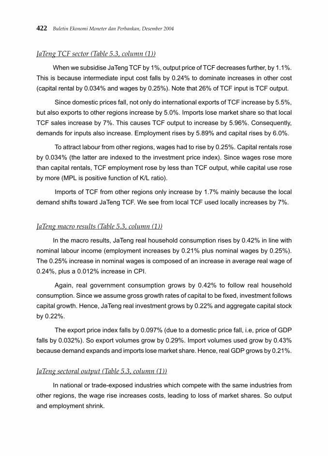
JaTeng TCF sector (Table 5.3, column (1))
When we subsidise JaTeng TCF by 1%, output price of TCF decreases further, by 1.1%.
This is because intermediate input cost falls by 0.24% to dominate increases in other cost
(capital rental by 0.034% and wages by 0.25%). Note that 26% of TCF input is TCF output.
Since domestic prices fall, not only do international exports of TCF increase by 5.5%,
but also exports to other regions increase by 5.0%. Imports lose market share so that local
TCF sales increase by 7%. This causes TCF output to increase by 5.96%. Consequently,
demands for inputs also increase. Employment rises by 5.89% and capital rises by 6.0%.
To attract labour from other regions, wages had to rise by 0.25%. Capital rentals rose
by 0.034% (the latter are indexed to the investment price index). Since wages rose more
than capital rentals, TCF employment rose by less than TCF output, while capital use rose
by more (MPL is positive function of K/L ratio).
Imports of TCF from other regions only increase by 1.7% mainly because the local
demand shifts toward JaTeng TCF. We see from local TCF used locally increases by 7%.
JaTeng macro results (Table 5.3, column (1))
In the macro results, JaTeng real household consumption rises by 0.42% in line with
nominal labour income (employment increases by 0.21% plus nominal wages by 0.25%).
The 0.25% increase in nominal wages is composed of an increase in average real wage of
0.24%, plus a 0.012% increase in CPI.
Again, real government consumption grows by 0.42% to follow real household
consumption. Since we assume gross growth rates of capital to be fixed, investment follows
capital growth. Hence, JaTeng real investment grows by 0.22% and aggregate capital stock
by 0.22%.
The export price index falls by 0.097% (due to a domestic price fall, i.e, price of GDP
falls by 0.032%). So export volumes grow by 0.29%. Import volumes used grow by 0.43%
because demand expands and imports lose market share. Hence, real GDP grows by 0.21%.
JaTeng sectoral output (Table 5.3, column (1))
In national or trade-exposed industries which compete with the same industries from
other regions, the wage rise increases costs, leading to loss of market shares. So output
and employment shrink.

423Illustrative Subsidy Variations to Attract Investors
However, industries less exposed to competition grow. For example, utilities grow by
0.40% and government services by 0.31%. Since local goods are produced and consumed
locally, demand for local goods grows to follow absorption (which is itself driven by labour
income). Since input costs to JaTeng firms rise, output prices also rise except in TCF sector.
Traded industries ranging from agriculture to manufactures shrink; machines and
electronics by 0.15% and mining by 0.16%. In turn, their demands for inputs contract.
Except for TCF exports, rising input costs cause exports to shrink. For example, in
agriculture domestic prices rise by 0.017% and exports shrink by 2.3%.
Jobs grow in TCF (by 5.9%) and in non-traded sectors, but shrink in trade-exposed
sectors.
5.5.2. Unfunded subsidy: effect on neighbour and nation
The effects on neighbour and nation of a long-run unfunded subsidy are shown in
Table 5.3, DIY (column (2)) and National (column (3)). Note that DIY is a neighbour region
surrounded by JaTeng. It is interesting to observe that effects on DIY are similar to effects
on JaTeng (but smaller). DIY also benefits, again led by increased TCF output. The reason
is that TCF partly from JaTeng is a big input into DIY TCF—so cheaper TCF imports benefit
DIY TCF also. National results are also positive, although small. One reason is that national
results are no more than the sum of the corresponding regional results.
TCF sector (Table 5.3, column (2, 3))
Since 24% of TCF in DIY is from JaTeng: a fall in JaTeng TCF domestic price by 1.1%
causes DIY TCF domestic prices to fall by 0.065%. As consequences, TCF output in DIY
expands by 0.57%. Then the demand of inputs rises, capital by 0.58% and labour by 0.55%.
To attract labour from other regions, wages had to rise by 0.077% relative to capital rentals
by 0.015% (the later are indexed to investment price index).
Due to TCF price falls, TCF output, export to ROW increases by 2.78%, and exports
to other regions increase by 0.75%. Import from other regions also increase by 1.6% because
of demand expansion. Again, local demand for local TCF rises by 0.11%.
Column (3) shows that national output prices for TCF falls by 0.16%. As results, TCF
output and exports all rise by 0.90% and by 1.42%. This sector sucks in employment from
other sectors by 0.90%. Note that national employment is fixed.

424 Buletin Ekonomi Moneter dan Perbankan, Desember 2004
Macro results (Table 5.3, column (2, 3))
In DIY, even though export prices fall by 0.031%, export volume falls by 0.046%. This
indicates that domestic demand is stronger than export. We can see from a rise in GDP
price index by 0.036%.
DIY also sucks in labour and capital from other regions. Aggregate employment and
capital stock in DIY increase by 0.029% and 0.021%. This causes real GDP to grow by
0.023%. Since labour income rises, household expenditures and government expenditure
all rise by 0.059%. Real investment grows by 0.016% to follow a growth in capital stock.
Again, import volume used increases by 0.095% to follow expansion in economy activity.
Tabel 5.3.Unfunded subsidy to TCF industry in JaTeng
(1) JaTeng (2) DIY (3) NationalDescriptionMain Macro Variable
RealHou Real Household Expenditure 0.418 0.059 0.001RealInv Real Investment Expenditure 0.219 0.016 0.001RealGov Real Government Expenditure 0.418 0.059 0.003ExpVol Export Volume 0.285 -0.046 0.027Xdomexp_c Export to other regions 0.261 0.060 -Xdomimp_c Import from other regions 0.378 0.058 -ImpVolUsed Import Volume Used 0.425 0.095 0.026ImpsLanded Import Volume Landed 0.332 0.130 0.026RealGDP Real GDP 0.206 0.023 0.001AggEmploy Aggregate Employment 0.208 0.029 0.000AveRealWage Average Real Wage 0.241 0.062 0.033AggCapStock Aggregate Capital Stock 0.220 0.021 0.002GDPPI Price GDP -0.032 0.036 0.000CPI Consumer Price Index 0.012 0.015 0.001ExportPI Export Price Index -0.097 -0.031 -0.012
DescriptionTCF Sector Variable
xexpsho(“TCF”) Direct exports to Row 5.533 2.776 1.416xtot(“TCF”) Industry output 5.962 0.565 0.902plab_o(“TCF”) Nominal wage 0.253 0.077 -xlab_o(“TCF”) Employment 5.892 0.547 0.898pcapsho(“TCF”) Capital rentals 0.034 0.015 -xcap(“TCF”) Capital 6.008 0.578 -pint(“TCF”) Intermediate cost -0.236 -0.120 -pdom(“TCF”) Domestic prices -1.111 -0.065 -0.160xdomexp(“TCF”) Export to other regions 4.975 0.747 -xdomimp(“TCF”) Import from other regions 1.732 1.574 -xdomloc(“TCF”) TCF made and used locally 7.000 0.108 -
425Illustrative Subsidy Variations to Attract Investors
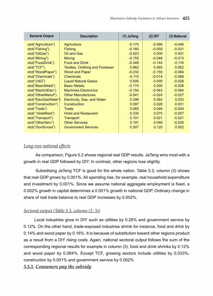
Long-run national effects
As comparison, Figure 5.2 shows regional real GDP results. JaTeng wins most with a
growth in real GDP followed by DIY. In contrast, other regions lose slightly.
Subsidising JaTeng TCF is good for the whole nation. Table 5.3, column (3) shows
that real GDP grows by 0.001%. All spending rise, for example, real household expenditure
and investment by 0.001%. Since we assume national aggregate employment is fixed, a
0.002% growth in capital determines a 0.001% growth in national GDP. Ordinary change in
share of real trade balance to real GDP increases by 0.002%.
Sectoral output (Table 5.3, column (2, 3))
Local industries grow in DIY such as utilities by 0.26% and government service by
0.12%. On the other hand, trade-exposed industries shrink for instance, food and drink by
0.14% and wood paper by 0.16%. It is because of substitution toward other regions product
as a result from a DIY rising costs. Again, national sectoral output follows the sum of the
corresponding regional results for example in column (3), food and drink shrinks by 0.12%
and wood paper by 0.084%. Except TCF, growing sectors include utilities by 0.033%,
construction by 0.001% and government service by 0.002%
5.5.3. Consumers pay the subsidy
(1) JaTeng (2) DIY (3) NationalDescriptionSectoral Output
xtot(“Agriculture”) Agriculture -0.170 -0.066 -0.046xtot(“Fishing”) Fishing -0.160 -0.059 -0.031xtot(“OilGas”) Oil and Gas -0.023 0.000 0.001xtot(“Mining”) Mining -0.155 -0.049 -0.013xtot(“FoodDrink”) Food and Drink -0.349 -0.144 -0.116xtot(“TCF”) Textiles, Clothing and Footwear 5.962 0.565 0.902xtot(“WoodPaper”) Wood and Paper -0.232 -0.155 -0.084xtot(“Chemicals”) Chemicals -0.110 -0.014 -0.066xtot(“LNG”) Liquid Natural Gases 0.000 0.000 -0.026xtot(“BasicMetal”) Basic Metals -0.174 0.000 -0.028xtot(“MachinElec”) Machines Electronics -0.154 -0.063 -0.064xtot(“OtherManuf”) Other Manufactures -0.041 -0.024 -0.027xtot(“ElecGasWater”) Electricity, Gas, and Water 0.396 0.262 0.033xtot(“Construction”) Construction 0.097 0.028 0.001xtot(“Trade”) Trade 0.065 0.048 -0.004xtot(“ HotelRest”) Hotel and Restaurant 0.335 0.075 -0.007xtot(“Transport”) Transport 0.101 0.021 -0.021xtot(“OtherServ”) Other Services 0.191 0.048 -0.026xtot(“GovSrvces”) Government Services 0.307 0.120 0.002

426 Buletin Ekonomi Moneter dan Perbankan, Desember 2004
In this section we subsidise the TCF industry by the same amount—this time funded
by a commodity tax on household purchases. Table 5.4 splits the results into three columns
showing, the effects of: (1) subsidy alone, (2) consumer tax, and (3) total.
To compute column (3) we allowed consumer taxes to adjust uniformly so that total
indirect tax revenue (including the subsidy cost) remained constant. The second column
shows the effect of the consumer tax increase alone. The necessary change was an increase
of 0.18% in the power of all taxes on household purchases. Column (1) is simply the difference
between (2) and (3). Due to model non-linearity it is not quite the same as column (1) of
Table 5.3.
Since the first column is nearly the same as the unfunded subsidy in the previous
section, here we focus on the second and total columns.
JaTeng macro results (Table 5.4, column (2))
A tax on households has opposing effects to an industry subsidy. All demand spending
in JaTeng went down, real household consumption by 0.26%, real investment by 0.082%
and real government consumption by 0.26%.
On the income side of GDP, aggregate employment falls by 0.13% and aggregate
capital stock by 0.082%. As a result real GDP shrinks by 0.097%. Since we assumed
capital/investment ratio to be fixed, investment also falls by 0.082%.
Figure 5.2Regional Real GDP Result

427Illustrative Subsidy Variations to Attract Investors
An increase on household power tax by 0.18% causes CPI to increase by 0.19%. In
turn, average real wages fall by 0.15%.
Due rising input costs, the export price index increases by 0.004% to cause a fall in
export volume by 0.10%. Again, import volume shrinks by 0.16% as a result of a shrinking in
production. The changes in export and import volumes hardly affect the real trade balance
to real GDP.
Tabel 5.4.Subsidy Funded by Consumer Tax (JaTeng Results)
(1) Efex of Subsidy
= (3) - (2)
(2) Efex of
Consumer Fax(3) TotalDescriptionMain Macro Variable
RealHou Real Household Expenditure 0.417 -0.258 0.159
RealInv Real Investment Expenditure 0.219 -0.082 0.137
RealGov Real Government Expenditure 0.417 -0.258 0.159
ExpVol Export Volume 0.286 -0.102 0.184
Xdomexp_c Export to other regions 0.261 -0.002 0.259
Xdomimp_c Import from other regions 0.378 -0.129 0.249
ImpVolUsed Import Volume Used 0.424 -0.158 0.266
ImpsLanded Import Volume Landed 0.331 -0.126 0.205
RealGDP Real GDP 0.206 -0.097 0.109
AggEmploy Aggregate Employment 0.208 -0.129 0.079
AveRealWage Average Real Wage 0.241 -0.149 0.092
AggCapStock Aggregate Capital Stock 0.220 -0.082 0.138
GDPPI Price GDP -0.032 0.132 0.100
CPI Consumer Price Index 0.012 0.187 0.199
ExportPI Export Price Index -0.097 0.004 -0.092
DescriptionTCF Sector Variables
xexpsho(“TCF”) Direct exports to ROW 5.530 -0.039 5.491
xtot(“TCF”) Industry output 5.958 -0.068 5.889
plab_o(“TCF”) Nominal wage 0.253 0.038 0.292
xlab_o(“TCF”) Employment 5.888 -0.079 5.809
pcapsho(“TCF”) Capital rentals 0.034 0.003 0.038
xcap(“TCF”) Capital 6.004 -0.061 5.943
pint(“TCF”) Intermediate cost -0.236 0.003 -0.233
pdom(“TCF”) Domestic prices -1.111 0.008 -1.103
xdomexp(“TCF”) Export to other regions 4.973 -0.027 4.946
xdomimp(“TCF”) Import from other regions 1.732 -0.068 1.664
xdomloc(“TCF”) TCF made and used locally 6.994 -0.112 6.882
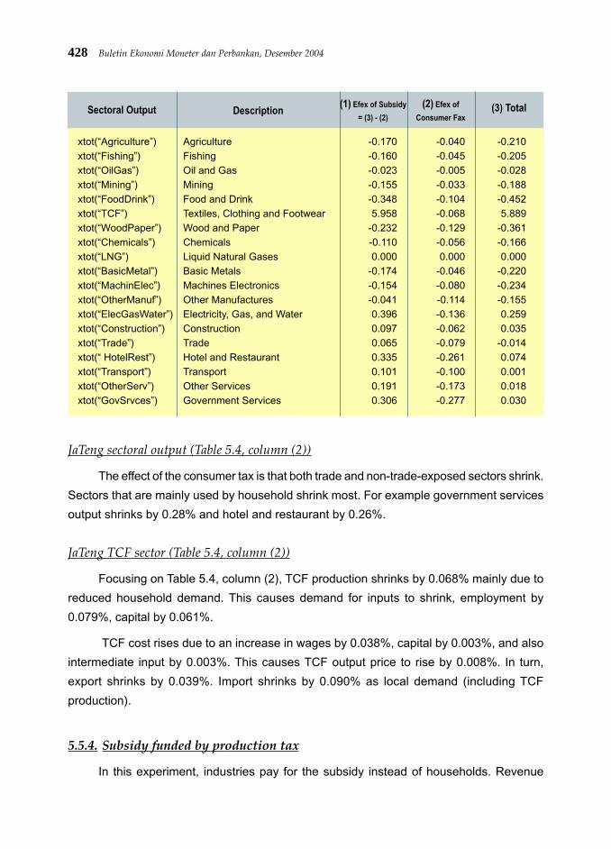
428 Buletin Ekonomi Moneter dan Perbankan, Desember 2004
JaTeng sectoral output (Table 5.4, column (2))
The effect of the consumer tax is that both trade and non-trade-exposed sectors shrink.
Sectors that are mainly used by household shrink most. For example government services
output shrinks by 0.28% and hotel and restaurant by 0.26%.
JaTeng TCF sector (Table 5.4, column (2))
Focusing on Table 5.4, column (2), TCF production shrinks by 0.068% mainly due to
reduced household demand. This causes demand for inputs to shrink, employment by
0.079%, capital by 0.061%.
TCF cost rises due to an increase in wages by 0.038%, capital by 0.003%, and also
intermediate input by 0.003%. This causes TCF output price to rise by 0.008%. In turn,
export shrinks by 0.039%. Import shrinks by 0.090% as local demand (including TCF
production).
5.5.4. Subsidy funded by production tax
In this experiment, industries pay for the subsidy instead of households. Revenue
(1) Efex of Subsidy
= (3) - (2)
(2) Efex of
Consumer Fax(3) TotalDescriptionSectoral Output
xtot(“Agriculture”) Agriculture -0.170 -0.040 -0.210
xtot(“Fishing”) Fishing -0.160 -0.045 -0.205
xtot(“OilGas”) Oil and Gas -0.023 -0.005 -0.028
xtot(“Mining”) Mining -0.155 -0.033 -0.188
xtot(“FoodDrink”) Food and Drink -0.348 -0.104 -0.452
xtot(“TCF”) Textiles, Clothing and Footwear 5.958 -0.068 5.889
xtot(“WoodPaper”) Wood and Paper -0.232 -0.129 -0.361
xtot(“Chemicals”) Chemicals -0.110 -0.056 -0.166
xtot(“LNG”) Liquid Natural Gases 0.000 0.000 0.000
xtot(“BasicMetal”) Basic Metals -0.174 -0.046 -0.220
xtot(“MachinElec”) Machines Electronics -0.154 -0.080 -0.234
xtot(“OtherManuf”) Other Manufactures -0.041 -0.114 -0.155
xtot(“ElecGasWater”) Electricity, Gas, and Water 0.396 -0.136 0.259
xtot(“Construction”) Construction 0.097 -0.062 0.035
xtot(“Trade”) Trade 0.065 -0.079 -0.014
xtot(“ HotelRest”) Hotel and Restaurant 0.335 -0.261 0.074
xtot(“Transport”) Transport 0.101 -0.100 0.001
xtot(“OtherServ”) Other Services 0.191 -0.173 0.018
xtot(“GovSrvces”) Government Services 0.306 -0.277 0.030

429Illustrative Subsidy Variations to Attract Investors
raised from production tax is used to subsidise the TCF sector. Again we split the results
into three columns: effect of subsidy, effect of production tax and total effect. To ease
comparison we also show in column (4), the total effect if consumers pay the subsidy (Table
5.5, column (4)). In this section we focus on the effect of the production tax (column (2)). To
pay for the TCF subsidy it was necessary to impose on all sectors a production tax equal to
0.066% of input costs.
JaTeng TCF sector (Table 5.5, column (2))
A rise in TCF production tax by 0.066% of output value only causes TCF domestic
prices to rise only by 0.047%. This is because regional wages fall by 0.23% to offset an
increase in capital rentals (by 0.012%) and intermediate input costs (by 0.015%). As TCF
output price increases, TCF output shrinks by 0.28%.
Due to a fall in output, TCF employment falls by 0.21% to depress local wage by 0.23%.
Increasing JaTeng commodity prices cause investment price index also to rise. Since we fixed
gross rate of return, rental price of capital also to rise by 0.012% to follow investment price
index. In turn, demand of capital falls by 0.33% as a result of an increase in capital rental.
Since TCF prices rises, exports to ROW shrinks by 0.20% and exports to other regions
shrinks by 0.189%. Import from other regions shrink by 0.14% because the substitution
effect is not enough to counteract the contraction in demand.
JaTeng macro results (Table 5.5, column (2))
Increases in most output prices cause all demand to fall. On the expenditure side of
GDP, real household and government expenditure fall by 0.41%, real investment falls by
0.30%, and export volumes fall by 0.62%. Since domestic demands fall, import volumes
also contract by 0.34%. Changes in export and import volume used causes share of real
trade balance to real GDP to increase by 0.001%
In spite of an increase in production tax by 0.07%, GDP price index only rises by
0.030%. It is because government price index falls by 0.053%, while other price indexes
rise, CPI by 0.005%, export price index by 0.024% and investment prices index by 0.012%
(recall capital rentals rise by 0.012%).
Government uses mainly government services (about 69% of government expenses).
Since government services is labour intensive sector. When local wage falls, so does the
output price. As consequences, government price index falls.

430 Buletin Ekonomi Moneter dan Perbankan, Desember 2004
On the income side of GDP, aggregate employment falls by 0.20% and aggregate
capital stock by 0.33%. Hence, real GDP shrinks by 0.26%.
JaTeng sectoral output (Table 5.5, column (2))
All sectors shrink to follow macro expenditure results. For example, government
services falls by 0.36% to follow a fall in real government spending by 0.41%. Construction
shrinks by 0.22% to follow a 0.30% fall in real investment expenditure.
Comparison with subsidy funded by consumer tax
Macro results indicate the production tax method of funding the TCF subsidy is far
more damaging to the JaTeng economy than the consumer tax. Raising the production tax
causes factor cost and intermediate costs to rise. As consequences, JaTeng demand
weakens. Even though export price index falls, this is not enough to raise the export. Imports
displace domestic products.
If producers pay for the subsidy, capital rentals rise by more than if the consumers pay
the subsidy. This offsets the effect of the subsidy on aggregate capital stock and causes it
and investment to fall. As a result, the real GDP shrinks when producers are taxed
Tabel 5.5.Subsidy funded by producer tax (JaTeng results)
RealHou Real Household Expenditure 0.417 -0.411 0.006 0.159
RealInv Real Investment Expenditure 0.219 -0.296 -0.077 0.137
RealGov Real Government Expenditure 0.417 -0.411 0.006 0.159
ExpVol Export Volume 0.292 -0.618 -0.326 0.184
Xdomexp_c Export to other regions 0.260 -0.090 0.170 0.259
Xdomimp_c Import from other regions 0.378 -0.318 0.060 0.249
ImpVolUsed Import Volume Used 0.425 -0.339 0.085 0.266
RealGDP Real GDP 0.206 -0.261 -0.054 0.109
AggEmploy Aggregate Employment 0.208 -0.201 0.007 0.079
AveRealWage Average Real Wage 0.241 -0.236 0.004 0.092
AggCapStock Aggregate Capital Stock 0.220 -0.329 -0.108 0.138
GDPPI Price GDP -0.032 0.030 -0.003 0.100
CPI Consumer Price Index 0.012 0.005 0.017 0.199
ExportPI Export Price Index -0.097 0.024 -0.073 -0.092
(1)
Efex of Subsidy
= (3) - (2)
(2)
Efex of
Consumer Fax
(3)TotalDescription
Main MacroVariable
(4)col (3), Table 5.4

431Illustrative Subsidy Variations to Attract Investors
The subsidy funded by producer tax causes employment to rise by less than when
funded by consumers.
5.5.5. Subsidy funded by reduction in local government demands
In this section our TCF subsidy is funded by a 2.19% reduction in local government
demand. Table 5.6 decomposes the results into two columns: effect of subsidy and effect of
government demand cut. We first discuss column (2): the effects of the government demand
DescriptionSectoral output
(1)
Efex of Subsidy
= (3) - (2)
(2)
Efex of
Consumer Fax
(3)TotalDescription
TCF SectorVariables
(4)col (3), Table 5.4
xexpsho(“TCF”) Direct exports to ROW 5.513 -0.202 5.311 5.491
xtot(“TCF”) Industry output 5.940 -0.279 5.661 5.889
plab_o(“TCF”) Nominal wage 0.253 -0.232 0.021 0.292
xlab_o(“TCF”) Employment 5.875 -0.207 5.668 5.809
pcapsho(“TCF”) Capital rentals 0.034 0.012 0.046 0.038
xcap(“TCF”) Capital 5.983 -0.328 5.655 5.943
pint(“TCF”) Intermediate cost -0.235 0.015 -0.221 -0.233
pdom(“TCF”) Domestic prices -1.111 0.047 -1.064 -1.103
xdomexp(“TCF”) Export to other regions 4.961 -0.189 4.772 4.946
xdomimp(“TCF”) Import from other regions 1.728 -0.144 1.584 1.664
xdomloc(“TCF”) TCF made and used locally 6.969 -0.374 6.595 6.882
xtot(“Agriculture”) Agriculture -0.169 -0.046 -0.215 -0.210
xtot(“Fishing”) Fishing -0.160 -0.056 -0.216 -0.205
xtot(“OilGas”) Oil and Gas -0.023 -0.067 -0.090 -0.028
xtot(“Mining”) Mining -0.155 -0.026 -0.181 -0.188
xtot(“FoodDrink”) Food and Drink -0.344 -0.391 -0.734 -0.452
xtot(“TCF”) Textiles, Clothing and Footwear 5.940 -0.279 5.661 5.889
xtot(“WoodPaper”) Wood and Paper -0.230 -0.484 -0.714 -0.361
xtot(“Chemicals”) Chemicals -0.110 -0.351 -0.461 -0.166
xtot(“LNG”) Liquid Natural Gases 0.000 0.000 0.000 0.000
xtot(“BasicMetal”) Basic Metals -0.174 -0.260 -0.433 -0.220
xtot(“MachinElec”) Machines Electronics -0.154 -0.319 -0.473 -0.234
xtot(“OtherManuf”) Other Manufactures -0.040 -0.340 -0.380 -0.155
xtot(“ElecGasWater”) Electricity, Gas, and Water 0.395 -0.293 0.103 0.259
xtot(“Construction”) Construction 0.097 -0.204 -0.107 0.035
xtot(“Trade”) Trade 0.066 -0.224 -0.157 -0.014
xtot(“ HotelRest”) Hotel and Restaurant 0.335 -0.430 -0.095 0.074
xtot(“Transport”) Transport 0.102 -0.261 -0.159 0.001
xtot(“OtherServ”) Other Services 0.191 -0.310 -0.119 0.018
xtot(“GovSrvces”) Government Services 0.307 -0.363 -0.056 0.030

432 Buletin Ekonomi Moneter dan Perbankan, Desember 2004
cut then discuss column (3): the total effects.
Since the first column is nearly the same as the unfunded subsidy in the previous
section, here we focus on the second and total columns.
JaTeng TCF sector (Table 5.6, column (2, 3))
Column (2), the effect of the government spending cut, shows that when government
releases labour and capital, wages fall by 0.11% and capital rentals fall by 0.013%. Also,
intermediate input cost falls by 0.012%. So, TCF output price falls by 0.025%. Then, output
expands by 0.13%. In turn, export to ROW and to other regions expand by 0.14% and by
0.13%. Import from other regions only expands by 0.009% due to substitution toward local
TCF (TCF produced and used locally increases by 0.13%).
Column (3), the total effect shows that TCF output grows by 6.1%. Government
spending cut can be interpreted as a subsidy to TCF sector by reducing production cost. In
comparison to the previous simulations, TCF domestic price under this policy falls by more,
1.14%. Consequently, TCF output, export to ROW and export to other regions all expand.
JaTeng macro results (Table 5.6, column (2))
Even though regional costs are decreasing, real household expenditure falls by 0.16%.
This is because JaTeng labour income decreases [Note that aggregate employment falls by
0.084% and real wage falls by 0.092% and 0.084% + 0.092% ~ 0.16%]. In contrast, real
investment grows by 0.052%, following a 0.05% growth in aggregate capital stock.
Since local prices decrease, export volumes increase by 0.44% (mainly to ROW) and
import volumes fall by 0.065%. The changes in exports and imports causes the share of real
trade balance in real GDP to grow by 0.016%.
Perhaps counterintuitively, the government cuts leads to a small GDP rise. This is
because we follow a rule6 that the average real wage and a labour migration elasticity
determine labour supply. If we apply an elasticity value of 3 (in this we used 1) real GDP
shrinks by 0.045%.
Falling wages induce JaTeng price indexes to fall. For example the CPI falls by 0.017%,
the export prices index by 0.016%, the investment price index by 0.013% and the government
price index by 0.052%, and so the GDP price index falls by 0.040%.
6 XLAB_IO(d)=AVEREALWAGE(d)^1*FLABSUP(d)*LABSLACK; where AVEREALWAGE(d)=average real wage; 1=labour migration elasticity; XLAB_IO(d)=inter-regional labour migration or labour supply; FLABSUP(d)=Labour migrationshifter; LABSLACK=Slack to allow aggregate employment constraint

433Illustrative Subsidy Variations to Attract Investors
Note that welfare cost of sacking government officers, for example teachers, are not
captured by this experiment.
JaTeng macro results (Table 5.6, column (3))
Column (3), the total effect, shows that all spending (except government) expand: for
example investment grows by 0.27%. JaTeng sucks in labour and capital— labour is up
0.12% and capital 0.28%. As a result, real GDP expands by 0.21%.
The export price index falls by 0.11%, but the CPI, only by 0.005%. This is because
the share of JaTeng TCF for export is about as twice as much for households. This causes
GDP price index to fall by 0.073%.
Since export price decreases, export volume increases by 0.73%. Again, import volume
expands by 0.36% as a result from expanding in production (driven by TCF sector).
JaTeng sectoral output (Table 5.6, column (2, 3))
Column (2), the effect of government spending cut, shows that government services,
hotel and restaurant, utilities and other services shrink because they released labours. On
the other hand, other sectors employed more labours so they grow.
Tabel 5.6.Subsidy funded by reduction in local government demands (JaTeng results)
(1) Efex of Subsidy
= (3) - (2)
(2) Efex of
gov cut(3) TotalDescriptionMain Macro Variable
RealHou Real Household Expenditure 0.416 -0.158 0.258
RealInv Real Investment Expenditure 0.219 0.052 0.271
RealGov Real Government Expenditure 0.408 -2.185 -1.777
ExpVol Export Volume 0.283 0.444 0.728
Xdomexp_c Export to other regions 0.262 0.093 0.355
Xdomimp_c Import from other regions 0.377 -0.063 0.314
ImpVolUsed Import Volume Used 0.424 -0.065 0.359
RealGDP Real GDP 0.206 0.000 0.206
AggEmploy Aggregate Employment 0.207 -0.084 0.124
AveRealWage Average Real Wage 0.240 -0.092 0.149
AggCapStock Aggregate Capital Stock 0.220 0.058 0.278
GDPPI Price GDP -0.033 -0.040 -0.073
CPI Consumer Price Index 0.012 -0.017 -0.005
ExportPI Export Price Index -0.097 -0.016 -0.113
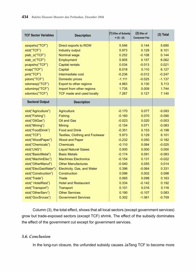
434 Buletin Ekonomi Moneter dan Perbankan, Desember 2004
Column (3), the total effect, shows that all local sectors (except government services)
grow but trade-exposed sectors (except TCF) shrink. The effect of the subsidy dominates
the effect of the government cut except for government services.
5.6. Conclusion
In the long-run closure, the unfunded subsidy causes JaTeng TCF to become more
(1) Efex of Subsidy
= (3) - (2)
(2) Efex of
Consumer Fax(3) TotalDescriptionTCF Sector Variables
xexpsho(“TCF”) Direct exports to ROW 5.546 0.144 5.690
xtot(“TCF”) Industry output 5.973 0.129 6.101
plab_o(“TCF”) Nominal wage 0.252 -0.108 0.144
xlab_o(“TCF”) Employment 5.905 0.157 6.062
pcapsho(“TCF”) Capital rentals 0.034 -0.013 0.021
xcap(“TCF”) Capital 6.018 0.110 6.127
pint(“TCF”) Intermediate cost -0.236 -0.012 -0.247
pdom(“TCF”) Domestic prices -1.111 -0.025 -1.137
xdomexp(“TCF”) Export to other regions 4.983 0.130 5.113
xdomimp(“TCF”) Import from other regions 1.735 0.009 1.744
xdomloc(“TCF”) TCF made and used locally 7.267 0.127 7.140
DescriptionSectoral Output
xtot(“Agriculture”) Agriculture -0.170 0.077 -0.093
xtot(“Fishing”) Fishing -0.160 0.070 -0.090
xtot(“OilGas”) Oil and Gas -0.023 0.020 -0.003
xtot(“Mining”) Mining -0.154 0.071 -0.083
xtot(“FoodDrink”) Food and Drink -0.351 0.153 -0.198
xtot(“TCF”) Textiles, Clothing and Footwear 5.973 0.129 6.101
xtot(“WoodPaper”) Wood and Paper -0.232 0.050 -0.182
xtot(“Chemicals”) Chemicals -0.110 0.084 -0.025
xtot(“LNG”) Liquid Natural Gases 0.000 0.000 0.000
xtot(“BasicMetal”) Basic Metals -0.174 0.091 -0.083
xtot(“MachinElec”) Machines Electronics -0.154 0.131 -0.022
xtot(“OtherManuf”) Other Manufactures -0.040 0.055 0.014
xtot(“ElecGasWater”) Electricity, Gas, and Water 0.396 -0.064 0.331
xtot(“Construction”) Construction 0.096 0.002 0.098
xtot(“Trade”) Trade 0.065 0.098 0.163
xtot(“ HotelRest”) Hotel and Restaurant 0.334 -0.142 0.192
xtot(“Transport”) Transport 0.101 0.016 0.116
xtot(“OtherServ”) Other Services 0.190 -0.107 0.083
xtot(“GovSrvces”) Government Services 0.302 -1.061 -0.759
435Illustrative Subsidy Variations to Attract Investors
competitive at the expense of other tradeable sectors. JaTeng sucks in labour (from other
regions) by 0.21% and capital by 0.22% (mainly from overseas). Real GDP grows by 0.21%.
National GDP also grows by 0.001%.
A subsidy funded by a households tax also raised JaTeng GDP (by 0.11%), but by
less than the unfunded subsidy. This is because the consumer tax weakens household
demand. JaTeng wins the most, followed by DIY (a region surrounded by JaTeng). Other
regions lose slightly because their workforce is moving to JaTeng and DIY, and because
they become unattractive to investors.
Taxing industries to finance the subsidy causes capital to flee JaTeng (fall 0.12%). As
a result real GDP shrinks by 0.054%. The reason is that the industry tax bears more heavily
on capital, which is in elastic supply.
If the subsidy is funded by a reduction in local government demands, labour moves
from government sectors to other more capital-intensive sectors especially tradeable sectors.
Real government spending shrinks but other spending grows more than in the previous
simulations. As a result, real GDP also grows by most, 0.206%, than the previous cases but
sacking government officers is not captured by this experiment.

436 Buletin Ekonomi Moneter dan Perbankan, Desember 2004
DAFTAR PUSTAKA
Abimanyu, Anggito (2000) “Impact of Agriculture Trade and Subsidy Policy on the
Macroeconomy, Distribution, and Environment in Indonesia: A Strategy for Future Industrial
Development”, The Developing Economies, Vol. XXXVIII, No. 4, pp. 547-71.
Adams, Philip D., J. Mark Horridge and Brian R. Parmenter (2000) “MMRF-GREEN: A
Dynamic, Multi-Sectoral, Multi-Regional Model of Australia”, Centre of Policy Studies
and Impact Project Preliminary Working Paper No. OP-94, Monash University, October.
May be downloaded from http://www.monash.edu.au/policy/elecpapr/op-94.htm
Armington, P.S. (1969) “The Geographic Pattern of Trade and the Effects of Price
Changes”, IMF Staff Papers, XVI, July, pp. 176-99.
Armington, P.S. (1970) “Adjustment of Trade Balances: Some Experiments with a
Model of Trade Among Many Countries”, IMF Staff Papers, XVII, November, pp. 488-523.
Dixon, P.B., B.R. Parmenter, J. Sutton and D.P. Vincent (1982) ORANI: A Multisectoral
Model of the Australian Economy (Amsterdam: North-Holland).
Hertel, T. W., and M. E. Tsigas, (1997): “Structure of GTAP”, in T. W. Hertel (ed.),
Global Trade Analysis: Modeling and Applications, Cambridge: Cambridge University Press.
Horridge, J.M., B.R. Parmenter and K.R. Pearson (1993) “ORANI-F: A General
Equilibrium Model of the Australian Economy”, Economic and Financial Computing, Vol. 3,
No. 2 (Summer), pp. 71-140.
Horridge, Mark (2000) “ORANI-G: A General Equilibrium Model of the Australian
Economy”, Centre of Policy Studies and Impact Project Preliminary Working Paper No. OP-
93, Monash University, October. May be downloaded from:http://www.monash.edu.au/policy/
elecpapr/op-93.htm